NLP with distrowatch reviews. Part III: Sentiment classification
Description
Some time ago, I contemplated transitioning to a Linux-based operating system, driven by my curiosity about the realm of free software and Linux culture. During my exploration, I stumbled upon the Distrowatch website (an invaluable resource offering information about numerous Linux distributions, including reviews). The organized and very structured layout of these reviews, coupled with the inclusion of numerical scores, sparked an idea within me. I envisioned gathering a substantial collection of these reviews—ranging from tens to potentially thousands—and subjecting them to analysis through Natural Language Processing (NLP). Eventually, this idea materialized into a tangible project, the outcome of which can be accessed here.
The project consists of three parts: Web scraping, supervised and unsupervised learning for sentiment analysis. We’ve already seen part I and II, let’s end with unsupervised learning.
Problem definition
In Part II, we categorized ratings using our intuition in order to differentiate between positive and negative reviews. However, this approach has a significant drawback, as it heavily depends on the subjectivity of the analyst, which in this case is me. Moreover, it introduces the potential for bias. Consequently, we will now explore alternative strategies for defining our target variable, mainly using unsupervised techniques.
Agglomerative clustering
What if we were to group categories/ratings based on the similarity of their features? To achieve this, we can generate a prototype exemplar for each rating and then apply a hierarchical clustering algorithm to group these representative members of each category. One relatively straightforward (although potentially simplistic) approach to creating a prototype for a rating/class $K$ is by calculating the average value of each feature across all instances with rating $K$.
The result of applying hierarchical clustering using cosine similarity and complete linkage is the following:
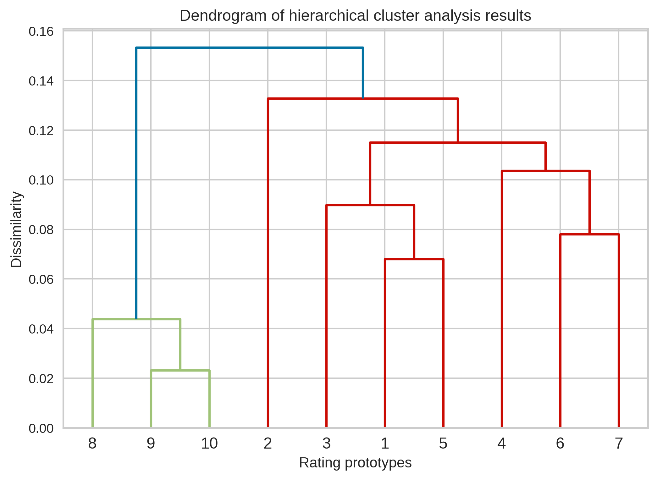
Interestingly, with this solution, we find ourselves in a situation where it makes sense to create two groups, roughly corresponding to positive reviews (ratings 8-10) and negative reviews (ratings 1-7). However, it’s worth noting that this classification is only approximate because intuitively, one might not consider a rating of 6 or 7 as entirely negative.
Using the two clusters as classes of the target variable, we can now train a model as we did in part II (same approach for text processing and data partition). Using Complement Naïve Bayes we get a global accuracy score of 0.844 and balanced accuracy of 0.828.
K-means
So far, in one way or another, the original rating data has been used to create the target variable. However, it is possible to take a completely unsupervised approach and generate the classes from the clusters that naturally emerge in the data. This can be achieved with K-means. Using this algorithm we can partition the dataset into a number of predefined groups and use the clusters ids as categories for supervised classification.
I decided to fit a model with two clusters because the elbow method didn’t help me choose the number of groups.The resulting clusters were completely (and therefore our target variable) new so I thought it would be reasonable to repeat the process of cross-validation for model selection. This time I introduced new models in the competetion: logistic regression and linear Support Vector Machine (SVM). The 5-cross-validation average balanced accuracy scores are show next:
| Model | Score |
|---|---|
| Complement Naïve Bayes | 0.638 |
| Logistic regression | 0.876 |
| Support Vector Machine | 0.956 |
Of course I chose SVM as the final model. In terms of test performance, this is what I got:
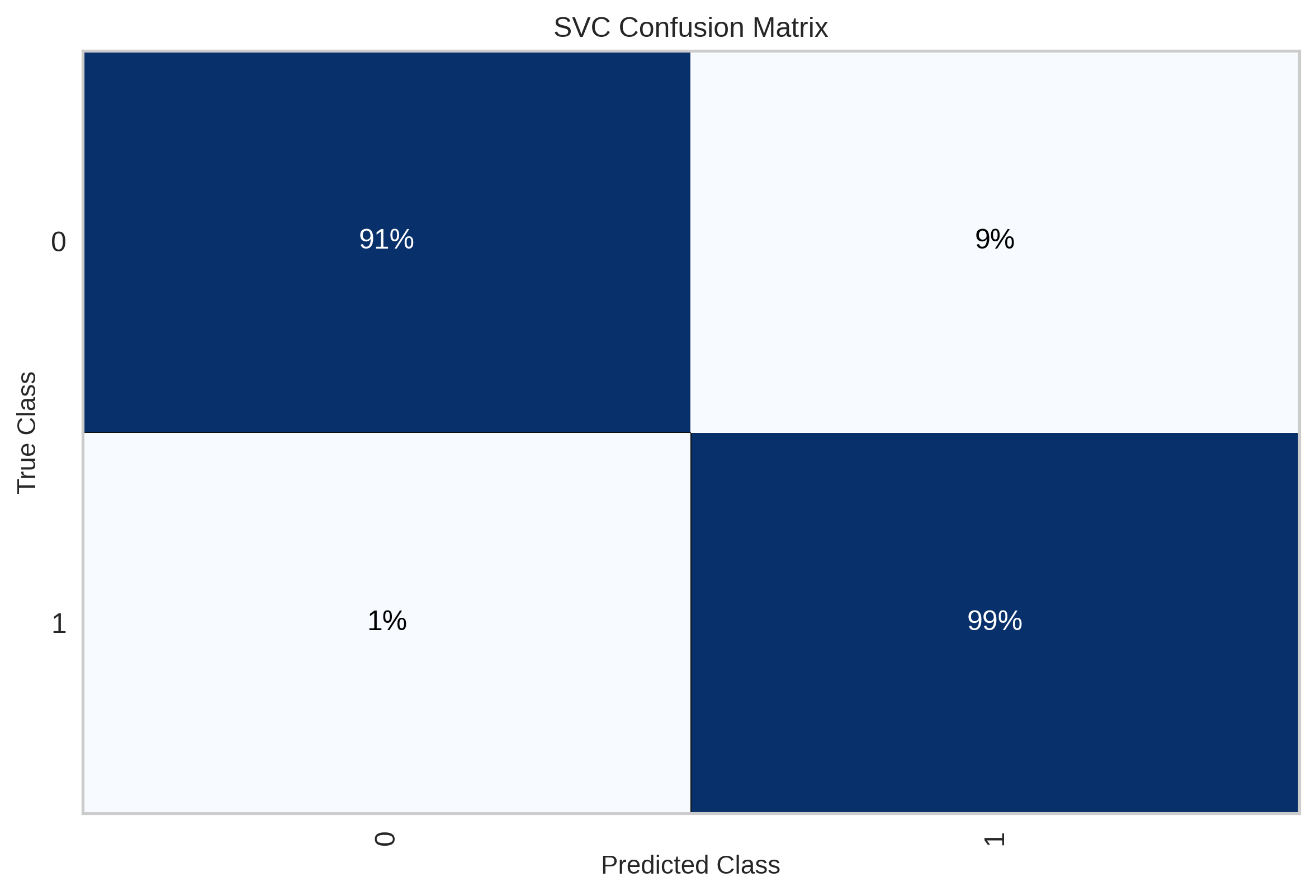
Pretty amazing, right? What happened here? What do the clusters represent? The model can be extremely good discriminating between classes, but if we don’t know the meaning of those classes, then the model is not useful at all. We hoped the categories could represent sentiment, is that really the case? Take a look at the distribution of ratings:
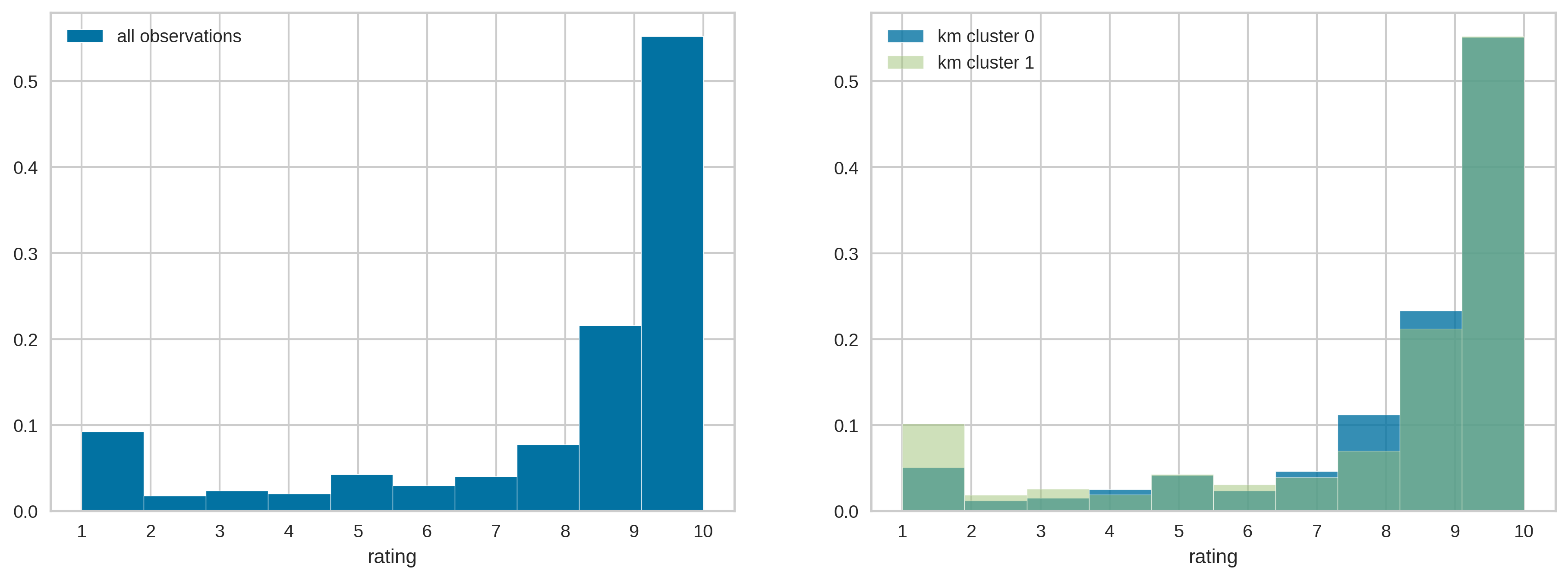
Mmm… I’m not sure. Yes, there is a higher proportion of low ratings (more evident with ratings of 1) in cluster 1 and a higher portion of very good reviews (8 or 9) in cluster 0, but the groups do not seem to be that distinct.
What about term frequency?
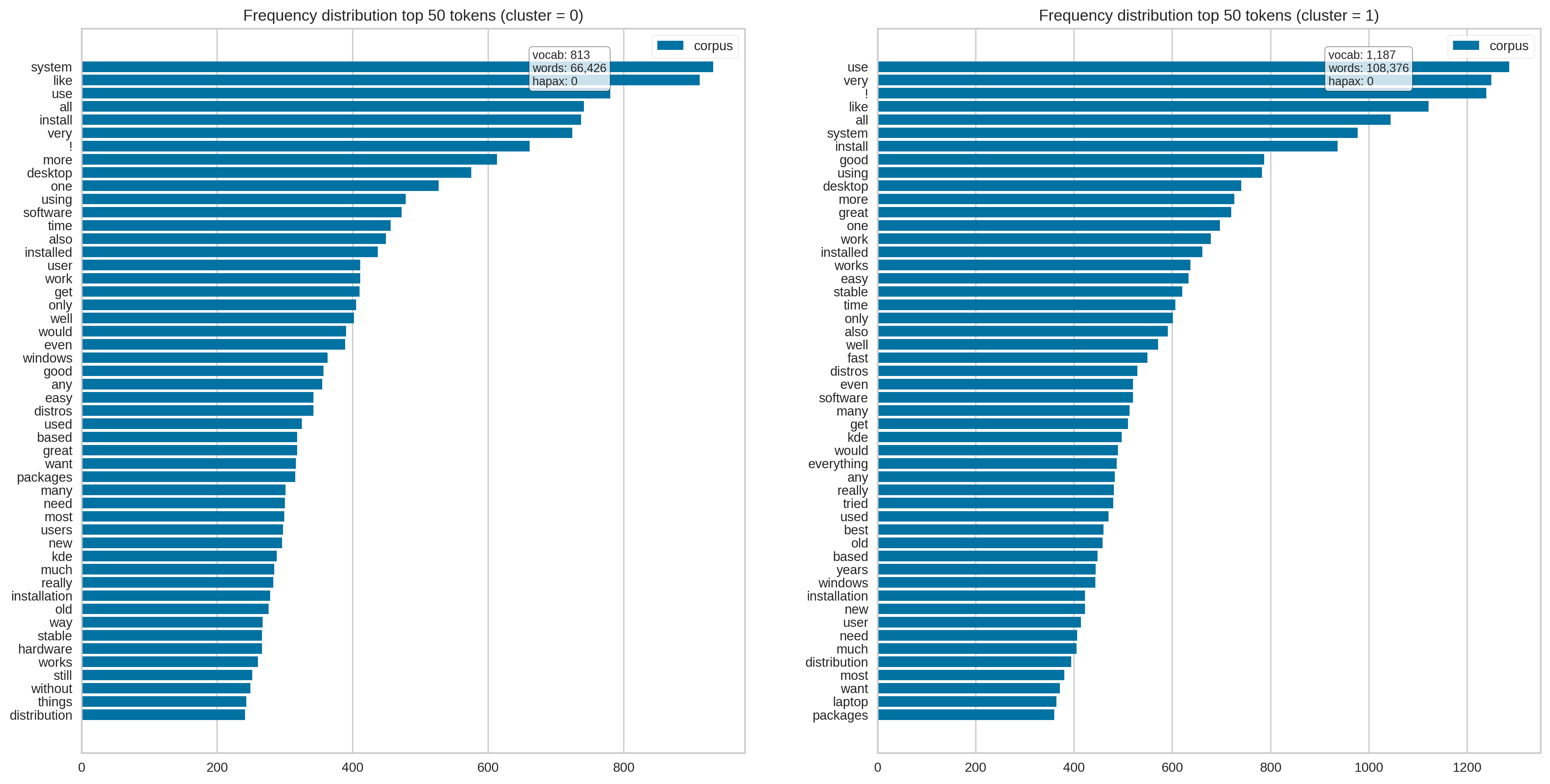
Not very clear.
Finally, taking advantage of the fact that we fit a linear classifier (they are usually easier to interpret), I examined the coefficients of the SVM
coefs = np.array(model['clf'].coef_.todense())
cl0_coefs,cl1_coefs = coefs[coefs<0],coefs[coefs>0]
top_cl0_tok,top_cl1_tok = cl0_coefs.argsort()[:10],np.flip(cl1_coefs.argsort()[-10:])
toks = model['vectorizer'].get_feature_names_out()

pd.DataFrame({
    'token cluster 0':toks[top_cl0_tok],
    'coef cluster 0':cl0_coefs[top_cl0_tok],
    'token cluster 1':toks[top_cl1_tok],
    'coef cluster 1':cl1_coefs[top_cl1_tok],
})
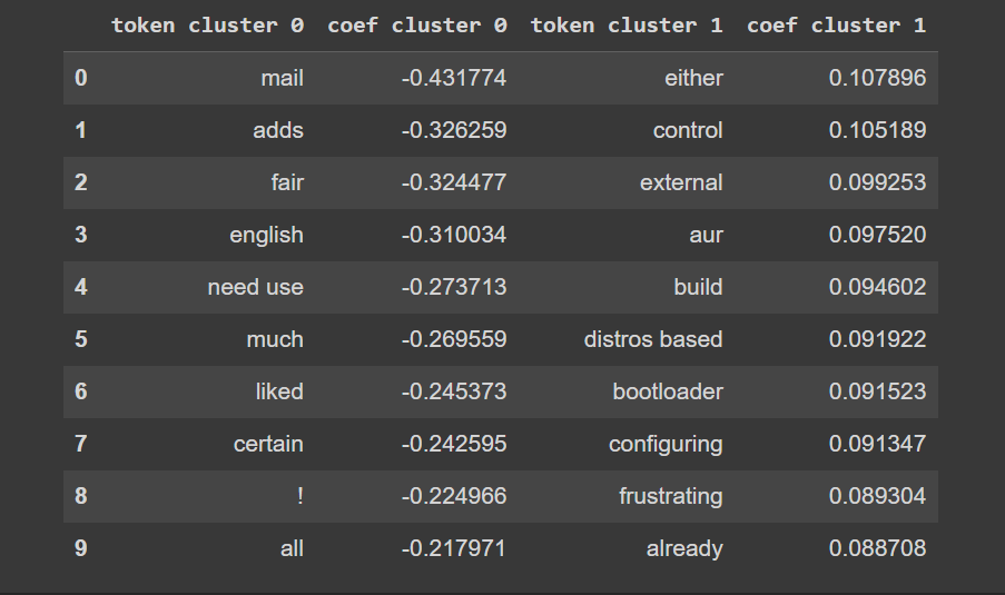
This is more interesting. Words like mail or adds have a strong influence on the decision boundary, meaning that the model relies more on them to classify the review, specifically into cluster 0. Generally, negative coefficients exhibit greater magnitude, which implies an emphasis on the “negative class”, which is cluster 0. This results in a skewed decision boundary favoring this class, which happens to be the minority class, by the way.
Still, I find difficult to give meaning to the clusters.
VADER
The last strategy to be considered involves the use of VADER (Valence Aware Dictionary and sEntiment Reasoner, consider checking the original paper or the implementation in nltk). This is a completely different approach, as VADER is a rule-based model that can itself be used as a classifier. It assigns scores to texts on a sentiment polarity scale ranging from -1 to 1 (-1 being the most negative, 1 being the most positive). Typically, a score of 0.5 or higher is considered to indicate positive sentiment, while a score of -0.5 or lower indicates negative sentiment, with the remaining scores reflecting neutrality.
When I applied it the first time I noticed a problem, however. It was clearly failing with many reviews. How do I know that? Well, remember that we had the real ratings given by the users. Now, let’s take a look at the distribution of scores in each category resulting from applying VADER:

It doesn’t seem logical that such a high proportion of ratings of 10 are classified as negative. Similarly, it’s also puzzling to find extreme cases (scores of 1 or 10) in reviews categorized as neutral.
For this reason, I then adopted a mixed approach where I utilized VADER but also took into consideration the information provided by the ratings. Specifically, VADER was only applied to reviews with ratings between 3 and 8. For the rest, which were clearly positive or negative, their scores were scaled to fit within the range of [-1, 1], and then the tag_review function was applied (see below). For VADER-rated reviews, the final sentiment score didn’t solely rely on VADER itself; it was a weighted combination of the VADER score and the scaled rating score:
$sentiment=\text{tag_review}(w\cdot VADER+(1-w)\cdot rating)$
def tag_review(compound_score):
  if compound_score >= 0.5:
    return 'pos'
  elif compound_score <= -0.5:
    return 'neg'
  else:
    return 'neu'
The new distributions seem more like what we would expect:

Then I repeated the model selection step. The results of the final Complement Naïve Bayes are shown next:

An unacceptable 68% of what we considered neutral reviews were classified as negative, and 24% were classified as positive reviews. This category caused considerable difficulty, so I considered reverting to the binary scenario. This was accomplished by simply altering the decision rule of VADER, that is, the tag_review function: scores $\geq$ 0 were positive, the rest, negative.
This lead to a new model that achieved 0.843 accuracy and 0.807 balanced accuracy, similar performance to what we saw earlier.
If you want to know more about the project, check the part I and II. All the code can be found here.