Prototype-based learning. Part I: GMLVQ from scratch
Description
In my journey to bridge psychology and data science, I discovered Learning Vector Quantization (LVQ) and immediately saw its potential connection to human category learning. This realization led me to dive deeper, implementing LVQ from scratch, initially by coding all the operations using PyTorch, and then by abstracting the optimization and learning processes to fully leverage PyTorch’s features.
Problem
Human category learning has been a subject of extensive study, with two predominant approaches: exemplar-based learning and prototype-based learning. Prototype learning, in particular, posits “that a category of things in the world (objects, animals, shapes, etc.) can be represented in the mind by a prototype. A prototype is a cognitive representation that captures the regularities and commonalities among category members and can help a perceiver distinguish category members from non-members” (Minda & Smith, 2011)
And what about LVQ? Well, this model learns prototypes and classifies new examples based on comparisons with these prototypes, which makes it a very promising model for human learning.
What is different and interesting?
One of the compelling aspects of LVQ is its flexibility in learning prototypes. Unlike traditional prototype models, which often rely on a single, average prototype per category, LVQ allows for multiple prototypes per category. These prototypes are not merely averages but can be more complex summaries of the data.
Furthermore, the similarity function in LVQ can be learned and adapted. Besides, this function doesn’t have to be unique; each prototype can have its own similarity function. This flexibility enables some LVQ models to handle not only linearly separable categories but also those that are non-linearly separable —a significant improvement over standard prototype models, which struggle with non-linear separations.
Objective
While LVQ shows promise as a cognitive model, validating it against human experimental data is beyond my current means due to a lack of access to such data. Therefore, my focus will be on evaluating LVQ’s effectiveness as a machine learning classifier. In this first part, I aim to replicate the results of a foundational paper in the LVQ field—the very paper that introduced me to this family of models (Schneider et al., 2009).
How to translate the model into code?
I’ve documented all the process in this report here and gathered all the code in this notebook.
Essentially, a trained LVQ model works by comparing an unseen exemplar ${\bf x}$ to each of the learned prototypes stored in memory ${\bf w}_1,…,{\bf w}_C$. There may be one for each of the $C$ classes, as here, or more than one. The comparison is done using a dissimilarity function $d$ defined as (assuming the use of row vectors instead of conventional column vectors):
$$ d({\bf x},{\bf w}_k,{\bf Q})=({\bf x}-{\bf w}_k) {\bf R} ({\bf x}-{\bf w}_k)^\intercal $$
Here, ${\bf R}_{p\times p}$ is relevance matrix. In GMLVQ, it’s a dense symmetric matrix of relevance/attention weights given to features where $tr({\bf R}) = 1$. If diagonal, the model will be Relevance LVQ (RLVQ) and won’t account for correlations between features. If identity matrix, we have the Generalized LVQ (GLVQ). When there is one matrix per prototype, we are working with localized versions of the model. In this first part of the project only GMLVQ and LGMLVQ are implemented. Also, this relevance matrix (or matrices) are expressed as ${\bf R}={\bf Q}^\intercal{\bf Q}$, so the dissimilarity becomes:
$$ d({\bf x},{\bf w}_k,{\bf Q})=({\bf x}-{\bf w}_k) {\bf Q}^\intercal{\bf Q} ({\bf x}-{\bf w}_k)^\intercal \ =\lVert {\bf Q}({\bf x}-{\bf w}_k)^\intercal \rVert_2^2 $$
The decision rule is to assign to the exemplar the class corresponding to the closest prototype:
$$ \hat c=\underset{k\in C}{\operatorname{argmin}}\ d({\bf x},{\bf w}_k,{\bf R}) $$
LVQ models learn the prototypes and the relevance matrix (or matrices) using gradient descent by minimizing the following relative distance loss:
$$ \mathcal{L}(d^+,d^-)=\phi\Bigl( \frac{d^+-d^-}{d^++d^-} \Bigr) $$
where $\phi$ is a function that can add an additional transformation. Here we are going to assume, as in the paper I’m using as reference, that $\phi(x)=x$, but in the second part we’ll try some other functions such as the sigmoid or ReLU. Notice that we have $d^+$ and $d^-$. Those distances are the distance of the data point from the closest prototype with the correct label (${\bf w}^+$) and the distance of the data point from the closest prototype with the incorrect label (${\bf w}^-$), respectively (from the energy-based model learning point of view, the latter would correspond to the “most offending answer”, a name that I found quite funny). In the “localized” model scenario, we would also have ${\bf R}^+$ and ${\bf R}^-$.
The tricky part when you implement a ML algorithm like this is that you need to code everything from scratch, including the derivatives (gradients) that are used for the parameter updates, so you need to understand very well how the model works. To save space, I won’t write here all the functions I created. If interested, check the report and/or notebook mentioned above.
Validation with artificial data
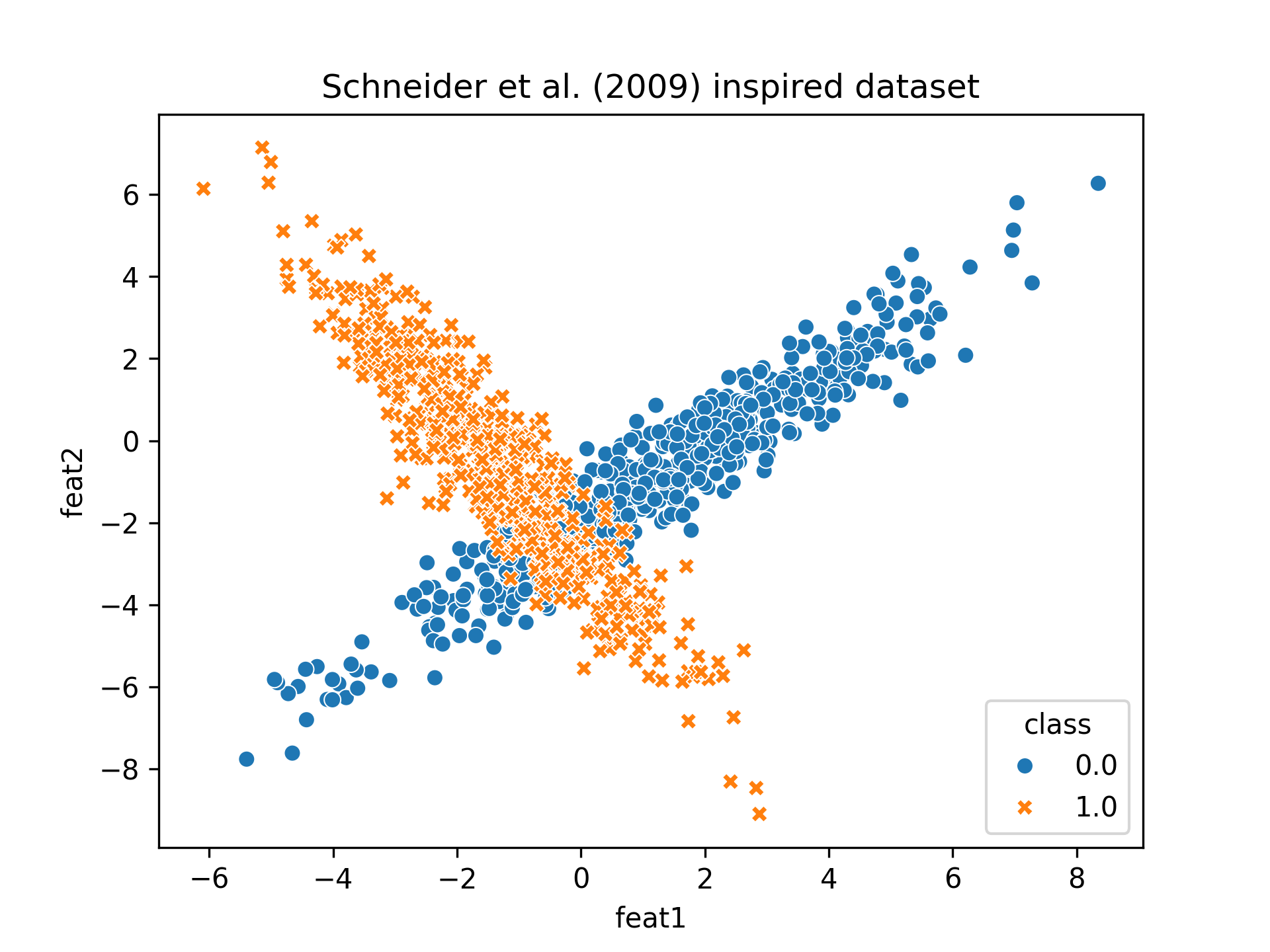
After having programmed the model, we’re ready to test it. In this first part we’ve only used a fake dataset with the same properties as the one generated in Schneider et al. (2009). It looks like this:
If we instantiate a GMLVQ model and train it for 25 epochs (way less that in the original paper, but there was no need of more epochs) we achieve around 0.8 accuracy which is pretty close to the one obtained in the paper. If we visualize the results we can see why tho model fails achieve higher accuracy.
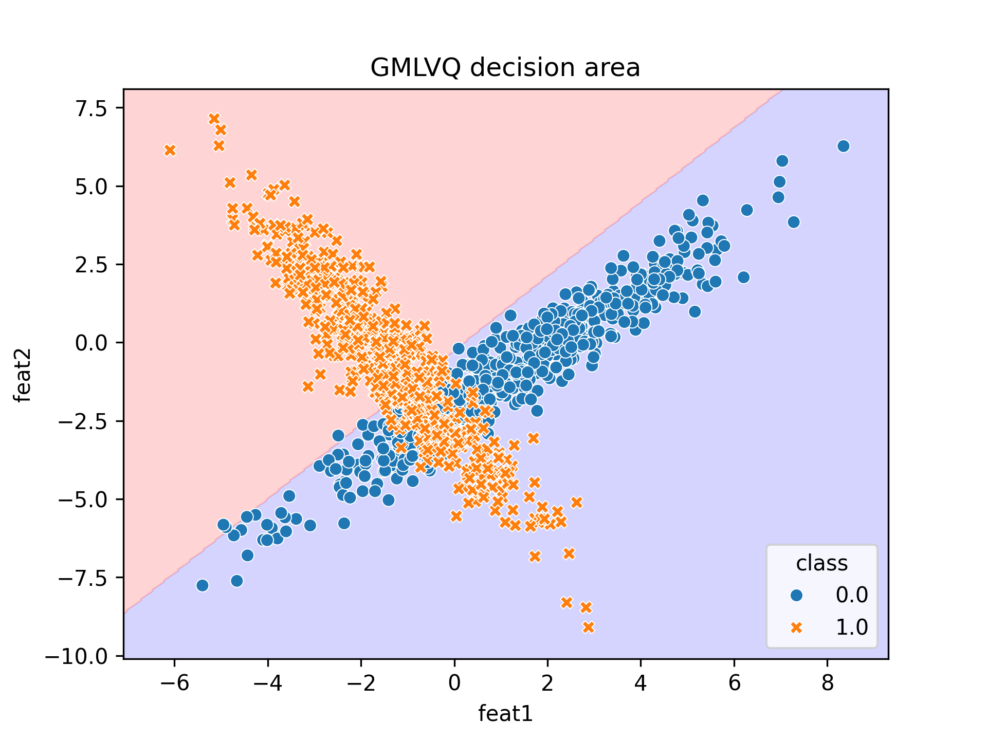
As said before (and much better explained in the paper, GMLVQ is at the end a linear classifier).
However, when we allow multiple relavance matrices with LGMLVQ, we obtain 0.91 accuracy and this is what we get.
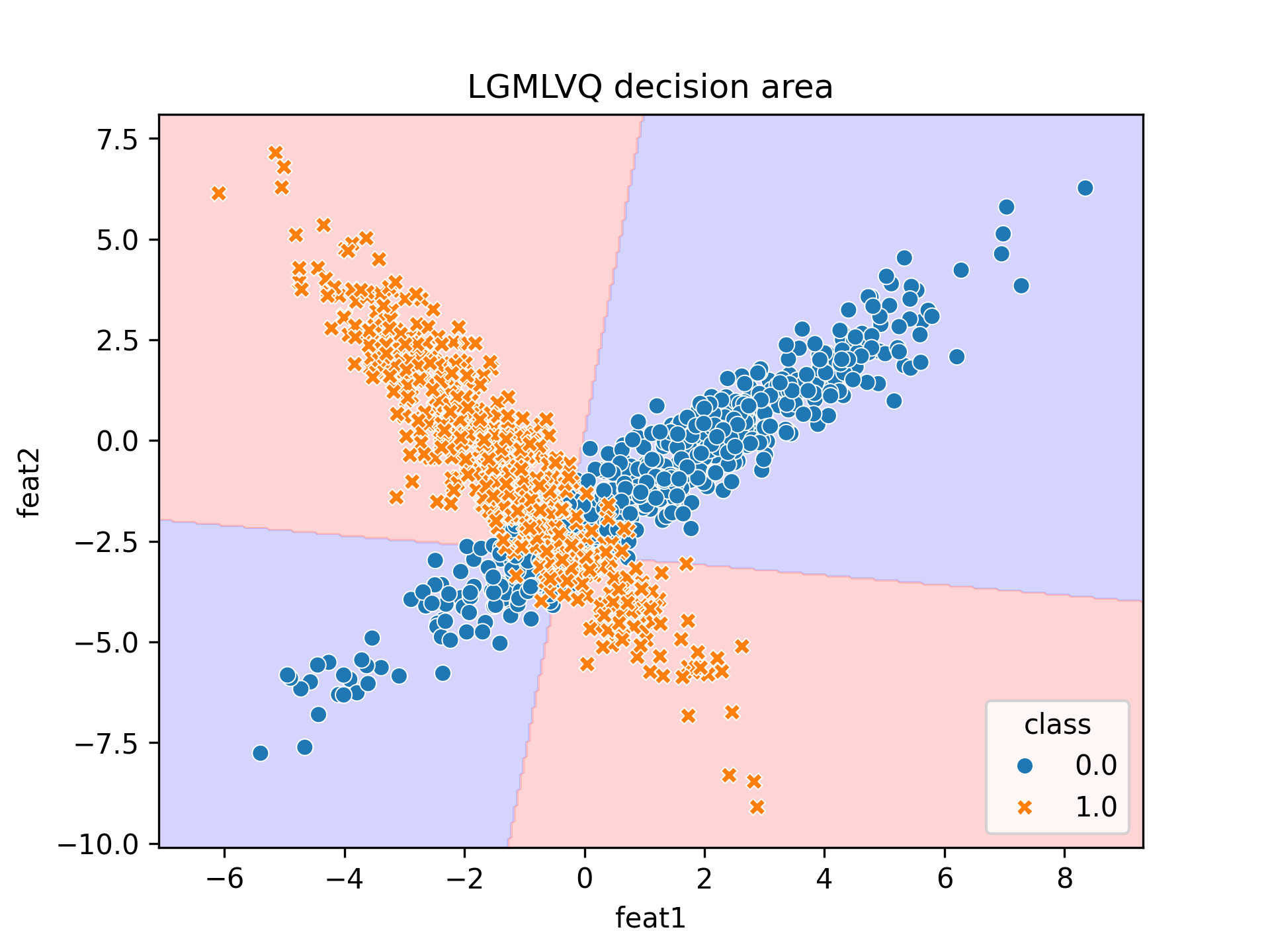
Nice, just as expected!
However, despite the success (I was very proud when I finally made it work), this was only the beginning, the code in this proof of concept was very rigid and didn’t allow for many changes. For that reason, just after I finished this I started working on a better version. Check it out in the second part !
References
Minda, J.P. & Smith, D. (2011). Prototype models of categorization: basic formulation, predictions, and limitations. In E.M. Pothos, N. Chater & P. Hines, Formal Approaches in Categorization (pp. 40-65)
Schneider, P., Biehl, M. & Hammer, B. (2009). Adaptive relevance matrices in Learning Vector Quantization, Neural computation, 21(12), 3532-3561.