Prototype-based learning. Part II: LVQ family of models in PyTorch
Description
In my journey to bridge psychology and data science, I discovered Learning Vector Quantization (LVQ) and immediately saw its potential connection to human category learning. This realization led me to dive deeper, implementing LVQ from scratch, initially by coding all the operations using PyTorch, and then by abstracting the optimization and learning processes to fully leverage PyTorch’s features.
In the previous part we showed how to create an (L)GMLVQ model totally from scratch, but it lacked several important features. Let’s now go one step further and try to re-implement it taking advantage of all PyTorch utilities.
From a set of independent functions to a PyTorch module
What we needed to do with several function calls, now is comfortably done just by instantiating an LVQ object with some parameters. The inner workings, however, remain practically the same. The most difficult part was that of integrating all LVQ variants functionalities within the same class. For instance, the same class should be able to instantiate an GLVQ model, which doesn’t require a relevance matrix, and also be capable of creating an GMLVQ model, which does require it. Other nuances were also taken into account, e.g. localized versions of LVQ require a slightly different distance function.
Finally, as a novel change, the possibility of using a limited rank pseudo-relevance matrix was implemented for (L)GMLVQ. By default, ${\bf R}_{p\times p}={\bf Q}{\bf Q}^\intercal$. This means that the pseudo-relevance matrix ${\bf Q}$ is also $p\times p$. However, we can reduce the number of parameters to be estimated (and, in a way, perform some kind of dimensionality reduction) by making ${\bf Q}_{p \times r}$, with $r \ll p$
class LVQ(nn.Module):
  """
    A class representing a Learning Vector Quantization (LVQ) model with various modes (GLVQ, GMLVQ, GRLVQ, LGMLVQ, etc.).
    The class supports different prototype initialization strategies and relevance matrices for generalized and local LVQ variants.

    Args:
        lvq_mode (str): The LVQ mode to use. Supported modes include:
        - 'glvq': Generalized LVQ.
        - 'gmlvq': Generalized Matrix LVQ.
        - 'grlvq': Generalized Relevance LVQ.
        - 'lgmlvq': Local Generalized Matrix LVQ.
        - 'lgrlvq': Local Generalized Relevance LVQ.

        data (torch.utils.data.TensorDataset): The dataset used for training, containing feature vectors and class labels.

        n_prototypes_per_class (list): A list where each element indicates the number of prototypes assigned to each class.

        naive_init (bool, optional): Whether to initialize the prototypes randomly (`True`) or based on class averages (`False`).
        Default is `False`.

       Q_rank (int, optional): The rank of the relevance matrix (Q) for local relevance LVQ variants. Default is `None`.

    Attributes:
        W (nn.ParameterList): The list of prototype tensors.
        prototype_labels (torch.Tensor): The class labels associated with each prototype.
        Q (nn.Parameter or nn.ParameterList): The relevance matrix/matrices used to compute distances between inputs and prototypes.
        distance_to_prototypes (callable): The distance function to compute distances between inputs and prototypes.
    """

  def __init__(self, lvq_mode, data, n_prototypes_per_class, naive_init=False, Q_rank=None):
    super(LVQ, self).__init__()
    self.lvq_mode = lvq_mode
    self.n_features = data.tensors[0].shape[1]
    self.n_prototypes = sum(n_prototypes_per_class)
    self.n_prototypes_per_class = n_prototypes_per_class
    self.W, self.prototype_labels = self.init_prototypes(data, naive_init)
    self.Q = self.init_pseudorelevance_matrix(Q_rank)
    self.distance_to_prototypes = self.choose_dist_function()

  def init_prototypes(self, data, naive_init):
    """
    Initializes the prototype vectors. Prototypes can be initialized either randomly (naive) or
    by averaging subsets of data points for each class.

    Args:
        data (torch.utils.data.TensorDataset): The dataset containing feature vectors and class labels.

        naive_init (bool): If `True`, prototypes are initialized randomly around the global average of the dataset.
        If `False`, they are initialized as class averages.

    Returns:
        nn.ParameterList: A list of initialized prototype vectors as parameters.
        torch.Tensor: A tensor containing the class labels associated with each prototype.
    """

    X, y = data.tensors
    W = []
    Wclasses = [[class_id] * times_each_proto for class_id, times_each_proto in enumerate(self.n_prototypes_per_class)]
    Wclasses = sum(Wclasses, []) # flattens nested list
    if naive_init:
      global_avg = X.mean(dim=0)
      W = [global_avg + torch.randn_like(global_avg) for _ in range(self.n_prototypes)]
    else:
      for class_id, times_each_proto in enumerate(self.n_prototypes_per_class):
        # get prototypes as avg of class
        for _ in range(times_each_proto):
          ids = torch.nonzero(y == class_id).squeeze()
          subset_size = (1/times_each_proto) * len(ids)
          subset_ids = ids[torch.randperm(len(ids))[:int(subset_size)]]
          w = X[subset_ids].mean(dim=0)
          W.append(w)

    return nn.ParameterList(W), torch.tensor(Wclasses).to(device)

  def init_pseudorelevance_matrix(self, Q_rank):
    """
    Initializes the (pseudo)relevance matrix (Q) based on the LVQ mode. In 'gmlvq' and 'grlvq', a global matrix is used, while
    in 'lgmlvq' and 'lgrlvq', local relevance matrices are used for each prototype.

    Returns:
        nn.Parameter or nn.ParameterList: The relevance matrix/matrices depending on the LVQ mode.
    """
    if Q_rank is None:
      Q_rank = self.n_features

    if self.lvq_mode == 'glvq':
      # Q = torch.sqrt(torch.eye(self.n_features))
      Q = torch.eye(self.n_features)

    elif self.lvq_mode == 'grlvq':
      Q = torch.sqrt(torch.eye(self.n_features))
      Q = nn.Parameter(Q)

    elif self.lvq_mode == 'gmlvq':
      Q = torch.randn((self.n_features, Q_rank))
      Q = Q / torch.sqrt((Q @ Q.T).diag().sum())
      Q = nn.Parameter(Q)

    elif self.lvq_mode == 'lgrlvq':
      Q = [torch.sqrt(torch.eye(self.n_features)) for _ in range(self.n_prototypes)]
      Q = nn.ParameterList(Q)

    elif self.lvq_mode == 'lgmlvq':
      Q = torch.randn((self.n_features, Q_rank))
      Q = [Q / torch.sqrt((Q @ Q.T).diag().sum()) for _ in range(self.n_prototypes)]
      Q = nn.ParameterList(Q)

    else:
      print('choose appropiate lvq model')
      return None

    return Q

  def choose_dist_function(self):
    """
    Selects the distance function based on the LVQ mode. The function computes the distance between input
    vectors and the prototypes, using either a global or local relevance matrix.

    Returns:
        callable: A function to compute the distances between input vectors and prototypes.
    """

    dists = []
    if self.lvq_mode == 'glvq':
      def distance_to_prototypes(x):
        dists = []
        for j in range(self.n_prototypes):
          raw_diff = x - self.W[j]
          d = torch.linalg.vector_norm(raw_diff, ord=2, dim=1, keepdim=True)**2
          dists.append(d)
        return torch.cat(dists, dim=1)

    elif self.lvq_mode == 'gmlvq' or self.lvq_mode == 'grlvq':
      def distance_to_prototypes(x):
        dists = []
        for j in range(self.n_prototypes):
          raw_diff = x - self.W[j]
          d = torch.linalg.vector_norm(raw_diff @ self.Q, ord=2, dim=1, keepdim=True)**2
          # d = torch.linalg.multi_dot([raw_diff, self.Q.t(), self.Q, raw_diff.t()])
          dists.append(d)
        return torch.cat(dists, dim=1)

    elif self.lvq_mode == 'lgrlvq' or self.lvq_mode == 'lgmlvq':
      def distance_to_prototypes(x):
        dists = []
        for j in range(self.n_prototypes):
          raw_diff = x - self.W[j]
          d = torch.linalg.vector_norm(raw_diff @ self.Q[j], ord=2, dim=1, keepdim=True)**2
          # d = torch.linalg.multi_dot([raw_diff, self.Q[j].t(), self.Q[j], raw_diff.t()])
          dists.append(d)
        return torch.cat(dists, dim=1)
    else:
      print('choose appropiate lvq model')

    return distance_to_prototypes

  def forward(self, x):
    """
     Forward pass for the LVQ model. Computes the distances between the input samples and the prototypes.

     Args:
         x (torch.Tensor): The input data, a tensor of shape (n_samples, n_features).

     Returns:
         torch.Tensor: A tensor containing the distances between each input sample and the prototypes.
    """

    dists = self.distance_to_prototypes(x)
    return dists
How does the model learn?
The implementation of the training algorithm has undergone significant changes. The most notable improvement is the elimination of the manual calculation of derivatives and updates. With the integration of autograd, we no longer need to explicitly code these calculations. Autograd automates the differentiation process, streamlining the training procedure and allowing us to focus on higher-level aspects of model design and optimization. This enhancement not only simplifies the implementation but also reduces the risk of errors in gradient calculations, leading to more reliable and efficient training.
def train_lvq(model, data_loader, epochs, loss_function, optimizer, scheduler=None, verbose=True):
  """
  Trains a Learning Vector Quantization (LVQ) model over a specified number of epochs using the provided
  data, loss function, and optimization strategy.

  Args:
      model (LVQ): An instance of the LVQ model that is being trained. The model contains prototypes,
      relevance matrices (Q), and the mode of training (e.g., 'gmlvq', 'lgmlvq', etc.).

      data_loader (torch.utils.data.DataLoader): A DataLoader object providing mini-batches of data (features `x`
      and labels `lab`) during training.

      epochs (int): The number of epochs to train the model for.

      loss_function (torch.nn.Module): The loss function to be used during training. Typically, this would be an instance
      of `GLVQLoss`, which computes the relative distance loss.

      optimizer (torch.optim.Optimizer): The optimizer responsible for updating the model parameters (prototypes and
      relevance matrices) based on the computed gradients.

      scheduler (torch.optim.lr_scheduler, optional): A learning rate scheduler that adjusts the learning rate during
      training, if provided. Defaults to `None`.

      verbose (bool, optional): Whether to print loss information after each epoch. If `True`, prints the average loss for each epoch.
      Defaults to `True`.

  Returns:
      None: The function updates the model parameters in place and prints loss information during training.

  Training Procedure:
      - For each mini-batch of data:
          1. Compute the distances between the input samples and the prototypes using the model.
          2. Identify the closest correct prototype (`d_pos`) and the closest incorrect prototype (`d_neg`) for each sample.
          3. Compute the loss using the provided `loss_function` (e.g., GLVQ loss).
          4. Perform backpropagation to compute the gradients.
          5. Update the model parameters (prototypes and relevance matrices) using the `optimizer`.
          6. If a `scheduler` is provided, adjust the learning rate after each step.
          7. Normalize the relevance matrices (`Q`) after each update to maintain their constraints.
      - After each epoch, print the average loss if `verbose` is set to `True`.

  Example:
      >>> model = LVQ('gmlvq', data, n_prototypes_per_class)
      >>> optimizer = torch.optim.SGD(model.parameters(), lr=0.01)
      >>> loss_fn = GLVQLoss(torch.nn.Identity())
      >>> train_lvq(model, data_loader, epochs=100, loss_function=loss_fn, optimizer=optimizer)

  Notes:
      - Different normalization steps are applied to the relevance matrix `Q` depending on the chosen LVQ mode:
          - 'gmlvq' and 'grlvq': Normalizes `Q` globally.
          - 'lgmlvq' and 'lgrlvq': Normalizes each relevance matrix individually.
  """

  model.train()
  for epoch in range(epochs):
    total_loss = 0.0
    for x, lab in data_loader:
      x, lab = x.to(device), lab#.to(device)
      optimizer.zero_grad()

      dists = model(x)
      d_pos = torch.stack([torch.min(dists[i, model.prototype_labels == lab[i]]) for i in range(len(lab))])
      d_neg = torch.stack([torch.min(dists[i, model.prototype_labels != lab[i]]) for i in range(len(lab))])

      loss = loss_function(d_pos, d_neg)
      total_loss += loss.item()
      loss.backward()
      optimizer.step()
      if scheduler is not None:
        scheduler.step()

      with torch.no_grad():
        if model.lvq_mode == 'gmlvq':
          model.Q.data = model.Q / torch.sqrt((model.Q @ model.Q.T).diag().sum())

        elif model.lvq_mode == 'grlvq':
          model.Q.data = torch.diag(torch.diag(model.Q.data))
          model.Q.data = model.Q / torch.sqrt((model.Q @ model.Q.T).diag().sum())

        elif model.lvq_mode == 'lgrlvq':
          for j in range(len(model.Q)):
            model.Q[j].data = torch.diag(torch.diag(model.Q[j].data))
            model.Q[j].data = model.Q[j] / torch.sqrt((model.Q[j] @ model.Q[j].T).diag().sum())

        elif model.lvq_mode == 'lgmlvq':
          for j in range(len(model.Q)):
            model.Q[j].data = model.Q[j] / torch.sqrt((model.Q[j] @ model.Q[j].T).diag().sum())

        else:
          pass

    if verbose:
      print(f"Epoch {epoch+1}/{epochs}, Loss: {total_loss/len(data_loader)}")

  return None
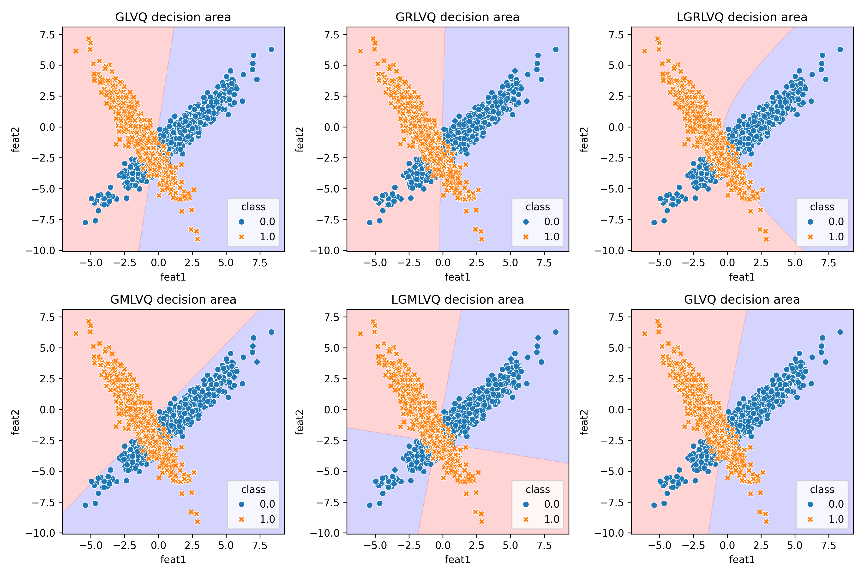
Validation with artificial data
With this new implementation, we are ready to revisit the artificial dataset from Schneider et al. (2009). This time, we can evaluate all the LVQ models as was done in the original experiments. Below are the results from our own LVQ implementation:
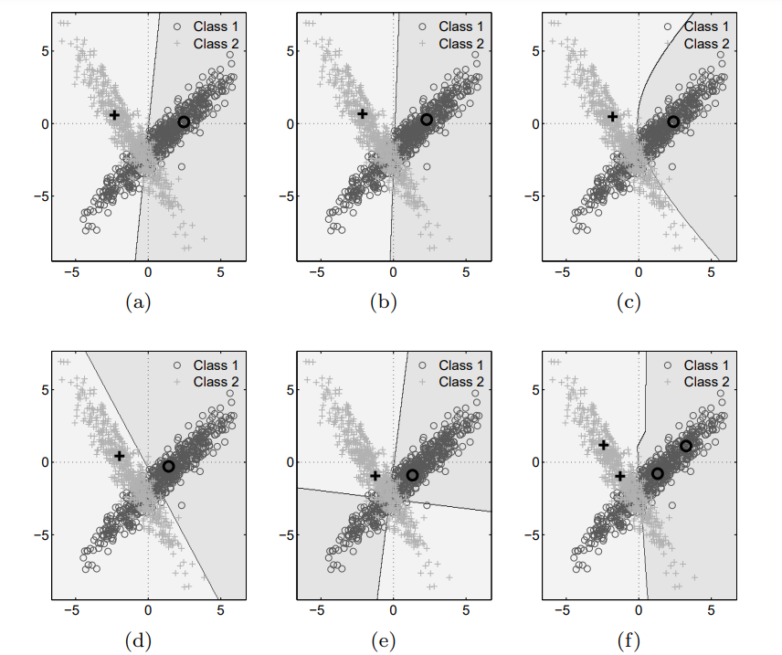
And this is what the authors obtained with their own (and a slightly different dataset)
Validation with artificial data
The first challenge has been successfully overcome, but now we need to return to our primary objective: assessing the effectiveness of LVQ as a machine learning classifier.
- Breast cancer
The breast cancer dataset serves as a critical benchmark for assessing the performance of LVQ in a practical and medically relevant setting. The dataset comprises 30 numeric features derived from diagnostic measurements, such as cell characteristics and histological attributes, to classify tumors into malignant or benign categories. This binary classification task presents a rigorous test for LVQ’s capability to not only classify instances accurately but also to discern meaningful patterns in the data.
model = LVQ('gmlvq', train_data, [1, 1])
loss_function = GLVQLoss(nn.ReLU()) # instead of the identity, we are now using ReLU
optimizer = torch.optim.SGD([
      {'params': model.W, 'lr': 0.01},
      {'params': model.Q, 'lr': 0.01}
  ])
scheduler = torch.optim.lr_scheduler.StepLR(optimizer, step_size=2, gamma=0.1)
train_lvq(model, train_dl, 20, loss_function, optimizer, scheduler, verbose=False)

acc = lvq_accuracy(model, Xtest, ytest)
Accuracy: 0.9386
Very good indeed! Very close to linear SVM (0.9649) and without much tweaking.
- Iris
Ok, this one is easy, but it has one property that shouldn’t be overlooked, it has more than two classes. LVQ can be naturally extended to a multiclass setting, let’s see if that also happens with out implementation.
model = LVQ('grlvq', train_data, [1, 1, 1]) # here is the little change to incorporate more than two classes
loss_function = GLVQLoss(nn.Identity())
optimizer = torch.optim.SGD(model.parameters(), lr=0.01)
train_lvq(model, train_dl, 10, loss_function, optimizer)

acc = lvq_accuracy(model, Xtest, ytest)
Epoch 1/10, Loss: -0.6931396275758743
Epoch 2/10, Loss: -0.7052224278450012
Epoch 3/10, Loss: -0.6970410794019699
Epoch 4/10, Loss: -0.7202270850539207
Epoch 5/10, Loss: -0.7116026654839516
Epoch 6/10, Loss: -0.7305767238140106
Epoch 7/10, Loss: -0.7281564772129059
Epoch 8/10, Loss: -0.7446763068437576
Epoch 9/10, Loss: -0.7445089370012283
Epoch 10/10, Loss: -0.7374046295881271
Accuracy: 1.0000
Well, you can’t do better than that…
- Apple quality
This dataset is not widely known, but I’ve chosen it because it illustrates problems where prototype learning, and LVQ in particular, can be highly beneficial. The dataset contains a few thousand apples, and the goal is to determine their quality (good vs. bad) based on numerical features such as size, weight, sweetness… Most classifiers can predict an apple’s quality given its characteristics, but they only provide this binary classification. In contrast, LVQ not only learns to distinguish between good and bad apples but also identifies prototypes for each quality category. From a company’s perspective, these prototypes can serve as valuable benchmarks or objectives.
model = LVQ('lgmlvq', train_data, [1, 1])
loss_function = GLVQLoss(nn.Sigmoid())

# check this out, we are not forced to always use vanilla gradient descent!
optimizer = torch.optim.RMSprop([
    {'params': model.W, 'lr': 0.01},
    {'params': model.Q, 'lr': 0.001}
])
train_lvq(model, train_dl, 20, loss_function, optimizer, scheduler=None, verbose=False)

acc = lvq_accuracy(model, Xtest, ytest)
Accuracy: 0.8275
Not bad, but it’s also true that other algorithms like SVM with radial basis function kernel perform better (0.9075).
- Digits (this digits dataset, not to be confused with MNIST)
How does the model work with images? Do we get useful prototypes? By applying prototype learning methods such as LVQ to this dataset, we can investigate if the model not only achieves high accuracy but also generates prototypes that offer clear, interpretable representations of each digit. These prototypes could be beneficial for understanding how the model perceives and distinguishes between different digits, providing deeper insights into the image classification process.
For this task we used the simpler GLVQ model first and achieved 0.9194 accuracy, far from the 0.9778 of SVM. However, the LVQ model allowed ourselves to get this interesting plot:
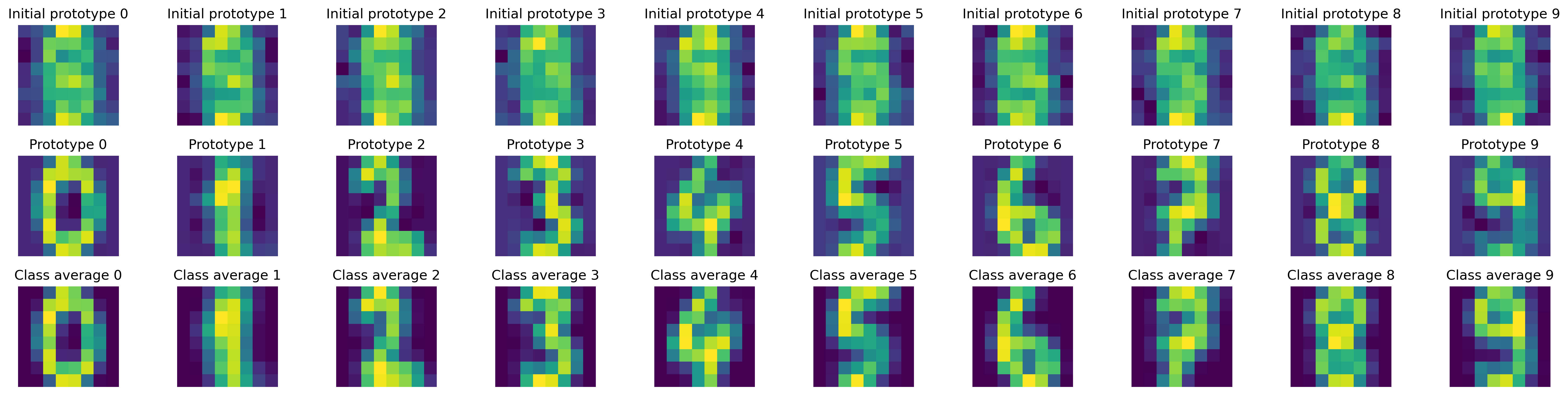
See that? Our “machine” began with a vague understanding of digits (we actually forced a naive initialization), but as it processed numerous examples from the dataset, it developed clear representations (prototypes) for each digit. Whenever it encounters a new digit, it retrieves these prototypes from memory and compares the new digit to them. By learning what digits like “2” or “5” typically look like, the machine can accurately classify new digits most of the time.
For those of you who might be disappointed with the initial performance of LVQ, don’t lose faith just yet. I also implemented a more complex LGMLVQ model and achieved an accuracy of 0.9806 (see the notebook for details).
- MNIST
Will the model work with high dimensional data and medium/large datasets? The model (at least some of the versions) work well with well with small datasets and less than 100 features, but in many situations we would need to deal with big datasets with way more features. Theoretical analysis anticipates that GMLVQ models are not a reasonable option in this cases because “computational costs [which] scale quadratically with the data dimensionality. Thus, quadratic instead of linear effort can be observed in every update step. Obviously, the method becomes computationally infeasible for very high dimensional data, i.e. 50 or more dimensions” (Schneider et al., 2009). In those situations, what can be done is adapt the matrix by “enforcing e.g. a limited rank of the matrix”. This means that ${\bf Q}$ is not $p \times p$, but $p \times r$, with $r \ll p$ ($p$ is the number of features).
Let’s try what happens with the MNIST dataset when using both GMLVQ alternatives
# full rank model: Q matrix is 784 x 784!
model_full = LVQ('gmlvq', train_data, prototypes_per_class, naive_init=False)
optimizer = torch.optim.Adam([
    {'params': model_full.W, 'lr': 0.01},
    {'params': model_full.Q, 'lr': 0.001}
])

start = time()
train_lvq(model_full, train_dl, 10, loss_function, optimizer, scheduler=None, verbose=True)
end = time()
print('Training time full rank model:', (end - start)/60)
acc = lvq_accuracy(model_full, Xtest, ytest)
Epoch 1/10, Loss: 0.060383220231555366
Epoch 2/10, Loss: 0.05668102145648154
Epoch 3/10, Loss: 0.05341387030132755
Epoch 4/10, Loss: 0.05151383971192797
Epoch 5/10, Loss: 0.04835201078282426
Epoch 6/10, Loss: 0.04789026859532654
Epoch 7/10, Loss: 0.04565780558801198
Epoch 8/10, Loss: 0.04361076997780862
Epoch 9/10, Loss: 0.04217445535974693
Epoch 10/10, Loss: 0.04022293095990996
Training time full rank model: 30.693514502048494
Accuracy: 0.7034
# limited rank model: Q matrix is just 784 x 20
model_lim = LVQ('gmlvq', train_data, prototypes_per_class, naive_init=False, Q_rank=20)
optimizer = torch.optim.Adam([
    {'params': model_lim.W, 'lr': 0.01},
    {'params': model_lim.Q, 'lr': 0.001}
])

start = time()
train_lvq(model_lim, train_dl, 10, loss_function, optimizer, scheduler=None, verbose=True)
end = time()
print('Training time limited rank model:', (end - start)/60)
acc = lvq_accuracy(model_lim, Xtest, ytest)
Epoch 1/10, Loss: 0.024052356710682624
Epoch 2/10, Loss: 0.019638755955913377
Epoch 3/10, Loss: 0.01786137058915677
Epoch 4/10, Loss: 0.01705550442239619
Epoch 5/10, Loss: 0.016361485048631826
Epoch 6/10, Loss: 0.01622419576663912
Epoch 7/10, Loss: 0.015414749924490859
Epoch 8/10, Loss: 0.014833231707938103
Epoch 9/10, Loss: 0.014462069061403841
Epoch 10/10, Loss: 0.01393588647092062
Training time limited rank model: 7.635886398951213
Accuracy: 0.8059
That’s impressive. Although neither of the models had fully converged yet and both still have room for improvement, we can draw some conclusions. Having fewer parameters not only drastically reduces computation time but also improves performance or, at the very least, increases the convergence rate.
Unfortunately, the limited-rank model is still somewhat slow and likely cannot compete with neural networks in terms of speed and scalability.
Known limitations
Even though we have managed to make the model work well in many situations, it is evident that it has some significant limitations as a machine learning model.
-
Tuning Complexity: Despite comparable performance with other machine learning models, LVQ requires much more extensive tuning. It demands adjustments similar to those needed for feedforward neural networks, such as batch size, learning rate, and training epochs. Furthermore, the results can be significantly influenced by these parameters, making careful tuning crucial for optimal performance.
-
Computational Cost: For GMLVQ, the computational effort grows quadratically rather than linearly with each update step. This poses a challenge, as the model is best suited for relatively small problems, typically with 10 to 50 features. However, this limitation may be less problematic upon further consideration. LVQ and its variants offer the advantage of providing prototypes learned from the data, which can be highly interpretable, especially when dealing with fewer features. Additionally, there is the option to work with rectangular matrices ${\bf Q}$ that have far fewer free parameters (as discussed in Bunte et al. (2008) and the final section of the notebook), which could mitigate some of the computational issues.
Link to code here.
References
Bunte, K., Schneider, P., Hammer, B., Schleif, F. M., Villmann, T., & Biehl, M. (2008). Discriminative visualization by limited rank matrix learning. Machine Learning Reports, 2, 37-51.
Schneider, P., Biehl, M. & Hammer, B. (2009). Adaptive relevance matrices in Learning Vector Quantization, Neural computation, 21(12), 3532-3561.