Random walks and decision making
What do the motion of particles in a medium (Brownian motion) and decision making have in common? Surprisingly enough, both phenomena can be mathematically modeled in the same way, as stochastic diffusion processes.
In psychology, the conceptual framework is more or less like this: A binary choice problem is presented to a decision maker, e.g., choose between candidate A and candidate B. We assume that the decision making process involves sequentially examining data samples (Wang & Busemeyer, 2021). We don’t know what kind of data is actually using the decision maker, but they serve as evidence favoring one or other alternative. In our voting example, we are assuming that the person is gathering information about the candidates, either explicitly and consciously (assessing the arguments given by each one) or implicitly and in a non-conscious way (being affected by peripheral cues such as attractiveness (see https://dictionary.apa.org/peripheral-cue)). It’s important to note that, obviously, we can’t observe the cognitive processes happening, so we cannot know what data the agent is assessing nor the value of the increment (incremented preference for A/B). However we can consider it as a process that varies randomly and model it probabilistically.
“The critical idea is that the decision-maker accumulates these evidence increments across time until the cumulative evidence becomes sufficiently strong (…)” (Wang & Busemeyer, 2021 p.122-23). Here, sufficiently strong means that the value representing the cumulative evidence reaches a threshold or decision criteria, so that a decision is finally made. After some time $t$ our voter will have enough information favoring A (or B) to choose A (or B).
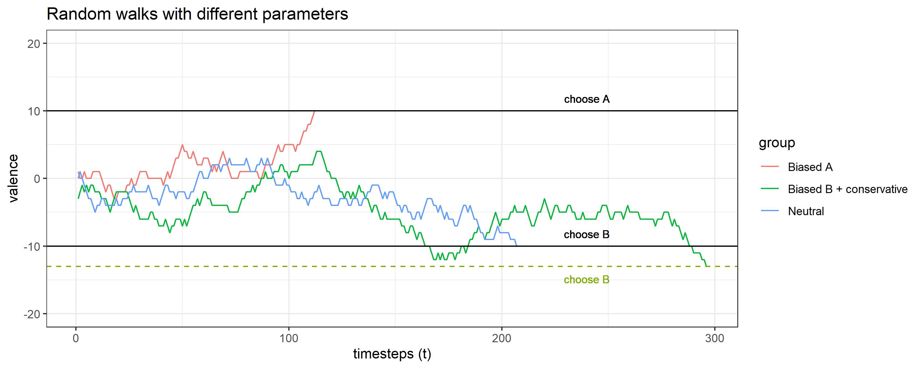
State-of-the-art models are rather complex and I just started learning about stochastic processes, but I find this area very interesting, so I decided to develop a very simple model, a random walk model. The algorithm is very basic. At every moment $t$, the agent can increment the “valence” for the alternative A by 1 point, increment the valence for B by 1 point (decrement the valence for A by -1) or stay the same. What really ends up happening every timestep depends on the probability of each possibility. At the same time, those probabilities are conditioned by some extra parameters. Specifically, the probability of encountering or sampling a piece of information that favors A depends on a sampling bias. Psychologically speaking, this could be some kind of memory bias. The bigger the bias, the more likely to encounter evidence that increments the valence. However, not every piece of information is accepted, the information can favor A, but we don’t necessarily consider it valid. The probability of accepting the evidence and updating the value of the valence is controlled by a acceptance bias. The bigger it is, the easier to accept the information as valid. A low bias might indicate some form of “reticence” or conservatism. The details are given in the report. But here are some results of simulating different “profiles”.

As we can see, when there is some preference for one of the alternatives, less time is needed to make a decision. Also, when the decision threshold is set significantly higher (in absolute value) comparing to other people, the response time increases.
From this random walk model we can make some interesting predictions. After some calculations we can obtain a formula that can let us predict the mean time needed to make a choice under some fixed conditions. If you want to know more, you can check the report.
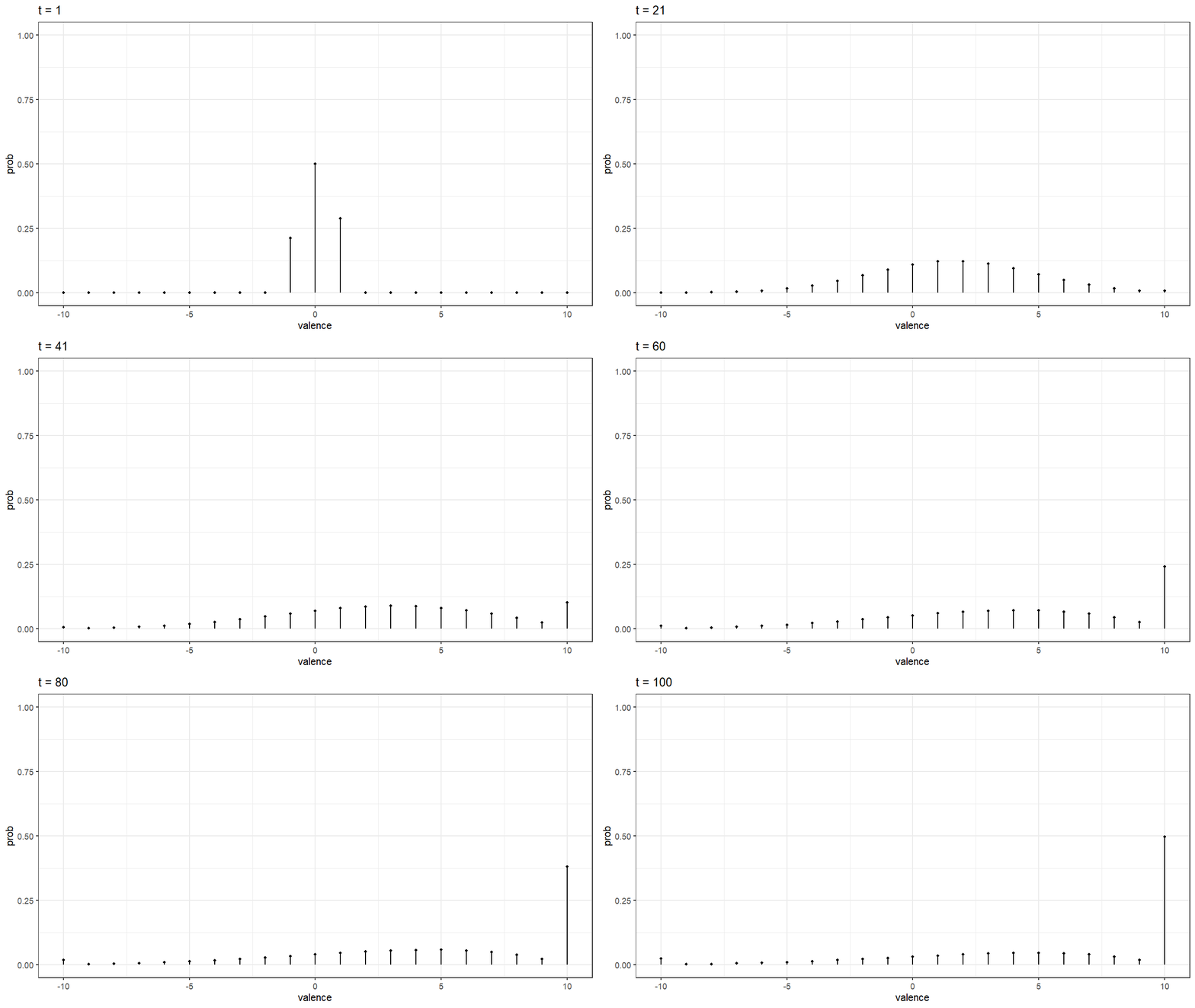
Finally, one of the things I found most exciting about these stochastic models, is that you can simulate something like the “development of the preference”. Imagine our decision maker has the decision boundary for A at 10, and the decision boundary at -10. That means that in order to choose A she needs accumulate evidence with a valence of 10. The same goes for B. In our model, that means there are 20+1 possible states or values of valence (counting 0). If we treat our random walk process as a Markov chain we can achieve some interesting predictions like knowing the probability of being in each state (valence) at any time. In the gif below we can see how this probabilities change as time goes on. Because the person simulated has some bias towards A, the probability distribution slowly shifts to the right, where valence for A is higher. By time $t=100$, the valence of 10 has the highest probability, indicating a clear preference and that the person have probably chosen A by that that time.

Full details of the algorithm, some of the mathematical details of the Markov chains and the R code can be found here