Is it normal?

Function to support the Kolmogorov-Smirnov test (for normality) graphically.

Description

A common task for many scientists, regarding data analysis, and especially in behavioral sciences, is to test if some variable of interest is normally distributed. One of the statistical techniques that is usually used is the Kolmogorov-Smirnov test (KS).It is based on the comparison of two distribution functions, one empirical ($F(Y_i)$), estimated from the collected data, and one theoretical ($F(Y_0)$). With KS we can test the null hypothesis that the empirical distribution is equal to the theoretical distribution, in this case, the normal distribution, with the parameters that we specify.

$$ \begin{aligned} H_0:F(Y_i)=F(Y_0) \end{aligned} $$

$$ \begin{aligned} H_1:F(Y_i)\neq F(Y_0) \end{aligned} $$

Eventhough this technique is very useful, it can be misleading sometimes because with big samples, even small deviations from normality are deemed statistically significant. To avoid dichotomic thinking (significant='bad’ and non-significant='good’), we can complement this test with some plots. Because KS is based on the comparison of two distribution functions, we can literally show this comparison by plotting the theoretical cumulative distribution function and the empirical distribution function. The goodness of fit can be assessed by looking if the two curves plotted overlap or not.

Code

def ks_test(Yi,mu,sigma):
    """
    Takes an array of values and returns its CDF and
    its theoretical CDF if it were normal. Also returns
    the value of the DKS statistic.

    Parameters
    ----------
    Yi : 1-D array-like (np.array or list)
        Vector of values that correspond to the observed values
        of our variable of interest.
    mu : int or float
        Expected value of the normal distribution we are testing.
    sigma : int or float
        Standard deviation of the normal distribution we are testing.

    Returns
    -------
    float.
        Value corresponding to the statistic DKS:
            DKS=max(abs(empirical_CDF - theoretical_CDF))

    """
    
    sorted_Yi=np.sort(Yi)
    emp_cdf=np.arange(start=1,stop=len(Yi)+1)/(len(Yi))
    theor_cdf=norm.cdf(sorted_Yi,loc=mu,scale=sigma)
    DKS=max(abs(emp_cdf-theor_cdf))
    
    fig,ax=plt.subplots()

    fig.suptitle('Kolmogorov-Smirnov visual test', fontsize=14, fontweight='bold')

    ax.scatter(sorted_Yi,emp_cdf,
               label='Empirical CDF',
               c='#ff6b6b',
               edgecolor='black',
               linewidths=.7,
              alpha=.8)
    ax.plot(sorted_Yi,emp_cdf,c='#ff6b6b',alpha=.4) # just to see the 'trajectory of the points'

    ax.scatter(sorted_Yi,theor_cdf,
               label='Theoretical CDF',
               c='#4ecdc4',
               edgecolor='black',
               linewidths=.7,
              alpha=.8)
    ax.plot(sorted_Yi,theor_cdf,c='#4ecdc4',alpha=.4) # just to see the 'trajectory of the points'

    if isinstance(Yi,pd.Series):
        ax.set_xlabel(Yi.name)
    else:
        ax.set_xlabel(r'$Y_i$')
    ax.set_ylabel('Cumulative probability')
    ax.legend(loc='center right');
    
    return DKS

Some examples

Imagine we want to know if newborns from mother who smoke tend to weigth less. Now imagine we can only collect data from 14 babies. It’s a very small sample, so we can’t rely on the Central Limit Theorem. Before trying to compare means or something like that, it would be necessary to check if we can assume that variable ‘weigth of newborns’ is normally distributed. We can quickly do that with the KS ‘visual’ test.

• Weigths corresponding to the 14 babies

Yi=np.array([1.48, 1.8, 1.93, 1.98, 2.04, 2.08, 2.18,
            2.2, 2.3, 2.45, 2.47, 3.15, 3.46, 4.64]) # data from Pardo & Ruiz (2015) pp.68

• Is the data normally distributed with mean equal to 2.5 and standard deviation equal to 1?

ks_test(Yi,mu=2.5,sigma=1)

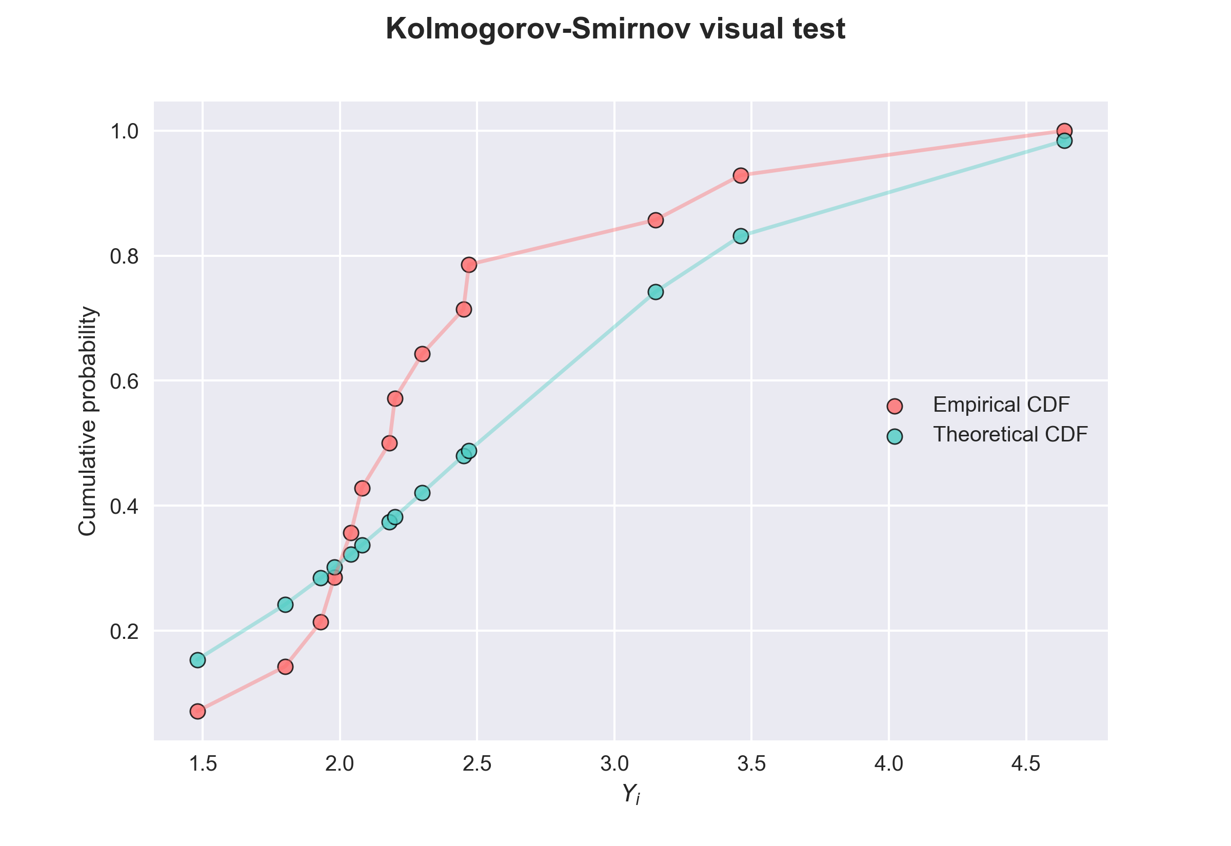
We can see that the data is clearly not normal.

Let’s look at another example. This one is made to show what happens when the variable is normal. We have a sample of 100 observations corresponding to scores in some recently developed intelligence test.

• IQ scores of 100 people

IQ=pd.DataFrame(np.random.normal(loc=100,scale=15,size=100),
                columns=['IQ Scores'])

• Are the scores of our test normally distributed with mean equal to 100 and standard deviation equal to 15?

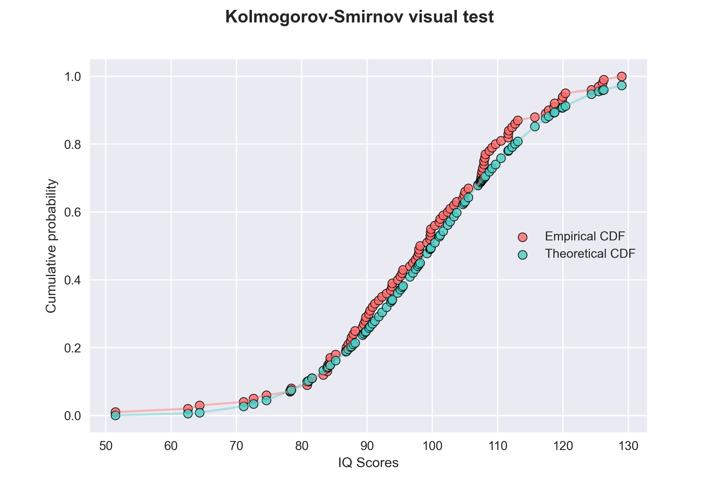
There is a great overlap, so we can conclude that the variable follows a normal distribution with $\mu$=100 and $\sigma$=15.

If you want to see the complete code, you can visit my Github profile.