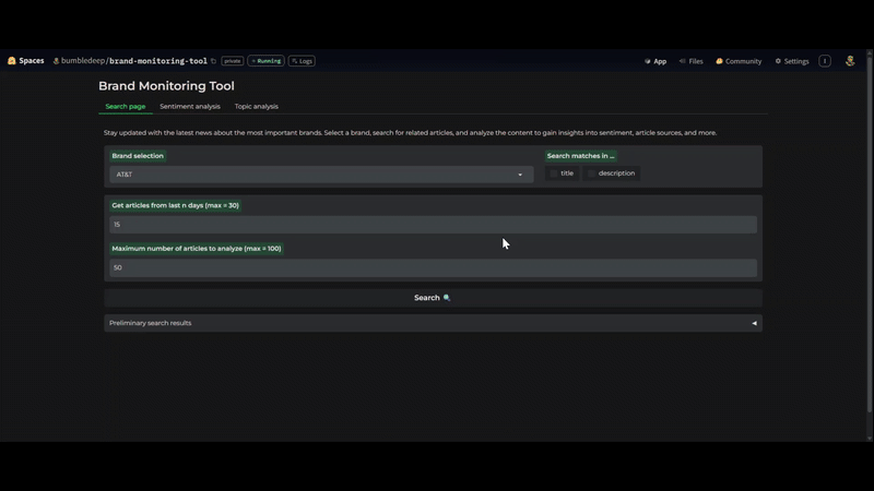
Monitor and analyze brands using language models

Description

I have built a brand monitoring application that leverages both large and specialized smaller language models. The entire application runs on CPU, relying on external APIs for specific tasks, making it a cost-free solution for users. While this minimizes monetary cost, the reliance on API limits and the absence of GPU acceleration naturally impose limitations on scalability.

Why This Project?

It all started with an exercise I did some time ago where I explored the capabilities of langchain and langgraph and developed an arbitrary text length summarizer using a small language model on scraped news articles. This experience ignited a desire to expand upon that initial concept, leading to the creation of an app that showcases the versatility and lightweight nature of specialized language models. The result is an effective OSINT (Open-Source Intelligence) tool designed for brand monitoring.

Development Workflow

1. Collecting Articles from the Web

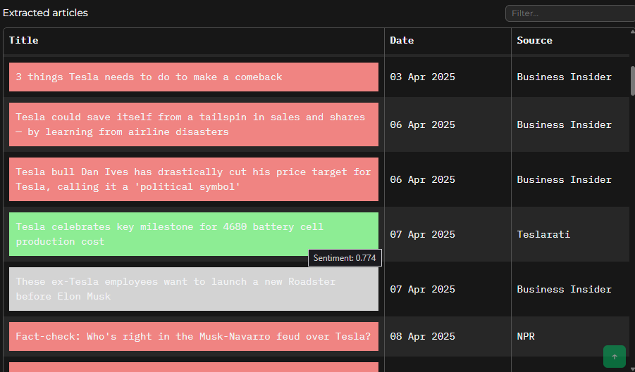
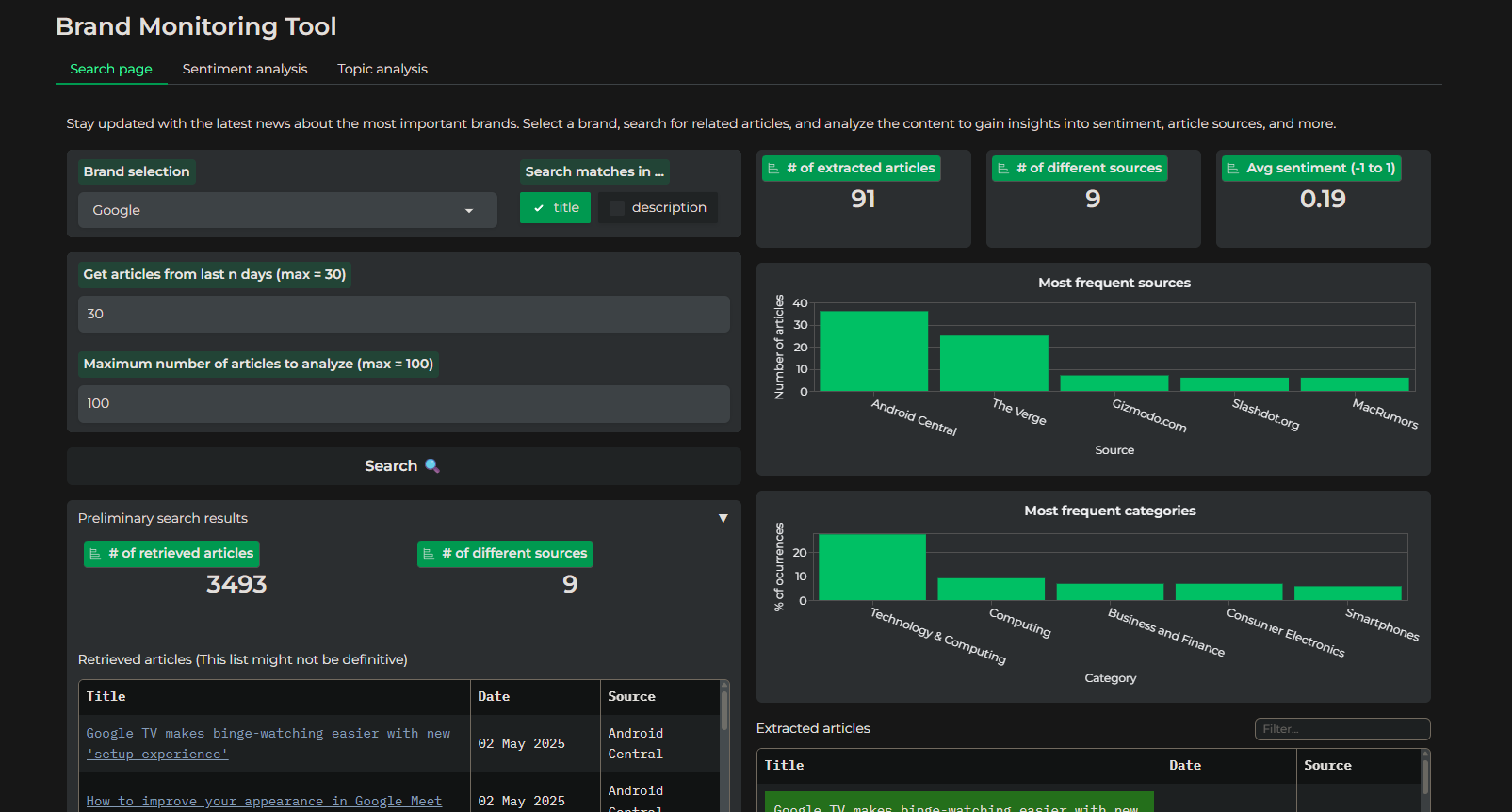
My primary tool for gathering news articles was the NewsAPI. It offers a highly useful set of filters, allowing for granular control over searches, such as excluding specific media sources, filtering by language, and focusing on matches within titles, descriptions, or the body of articles. However, a notable limitation is its “black box” nature; there’s no transparency regarding the internal search processes or how relevance is calculated when sorting articles. The problem with this is that I loose some control over the generated results. As an example, in the demo app you can see that when searching for “Tesla” articles, some completely irrelevant articles were included.

# API endpoint and parameters
newsapi_url = (
      'https://newsapi.org/v2/everything?'
      f'q={search_query}'
      f'&language={LANG}'
      f'&searchIn={search_in}'
      f'&from={from_date}'
      f'&to={today}'
      f'&excludeDomains={EXCLUDED_SOURCES}'
      '&sortBy=relevancy'
      f'&apiKey={NEWS_API_KEY}'
      )

2. Extracting Content from Articles

A significant discovery during this project was the Diffbot API. Beyond its core functionality of extracting content from a given URL, it also provides robust NLP capabilities, including summarization and sentiment scoring. This streamlined my workflow considerably.

# API endpoint and parameters
diffbot_api_url = (
        f'https://api.diffbot.com/v3/article?url={url}'
        f'&token={DIFFBOT_API_KEY}'
        f'&naturalLanguage=categories,sentiment,summary'
        f'&summaryNumSentences=4'
        f'&discussion=false'
    )

3. Sentiment Analysis

Initially, I planned to implement the summarization and sentiment scoring steps myself. However, upon discovering the Diffbot NLP API, I opted to integrate it due to its convenience. By simply adding a few extra parameters to the existing content extraction requests, I obtained excellent results. The major drawback, however, is Diffbot’s lack of transparency regarding its NLP API’s internal workings. The models used, the processing of full articles versus subsets, and any preprocessing steps remain undisclosed. Besides, there is not much room for customization, something that reduced the possibility of adapting the process to my usecase. Despite this, the quality of the results and the time saved made this a worthwhile compromise.

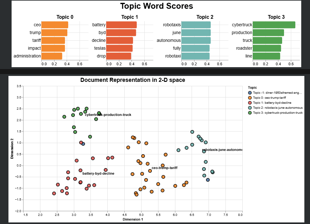
4. Topic Analysis

This was arguably one of the most challenging aspects of the project, primarily because I had to make a lot of decisions in terms of implementation. I adopted the BERTopic framework, another valuable discovery. This powerful framework comprises several stages:

• Embed documents: Converting text into numerical representations.
• Dimensionality reduction: Reducing the complexity of these embeddings.
• Cluster documents: Grouping similar documents together.
• Bag-of-words: Creating a representation of word frequency within clusters.
• Topic representation: Identifying the set of representative terms and documents of each cluster, as well as assigning meaningful labels to the identified clusters.

class CustomTokenizer(BaseTokenizer):

  def tokenize(self, text: str) -> list[str]:
      """Apply sklearn regex pattern to extract words"""

      words = findall(r"(?u)\b\w\w+\b", text)
      return words
      
def custom_tokenizer(text) -> list:
  """Custom tokenizer to remove plural nouns (with exceptions) and lemmatize verbs"""

  plural_exceptions = {"police", "data", "fish", "sheep", "species", "news", "media"} # exceptions suggested by chatgpt
  blob = TextBlob(text, tokenizer=CustomTokenizer())

  return [
      word.singularize() if tag == 'NNS' and word not in plural_exceptions
      else word.lemmatize(pos='v') if tag.startswith('V')
      else word
      for word,tag in blob.tags
  ]



def initialize_bertopic_components(n_docs: int, random_seed: int) -> dict:
  """Initializes and returns a dictionary of BERTopic model components.

  This function sets up the various models required for BERTopic, including
  the embedding model, dimensionality reduction, clustering, vectorization,
  c-TF-IDF, and representation models.

  Args:
      n_docs (int): The number of documents to be processed, used to determine
                    the minimum cluster size for HDBSCAN.
      random_seed (int): A seed for reproducibility in models that involve
                          randomness, such as UMAP.

  Returns:
      dict: A dictionary containing initialized instances of the BERTopic components:
            'embedding_model' (SentenceTransformer),
            'dimensionality_reduction_model' (UMAP),
            'clustering_model' (HDBSCAN),
            'vectorizer_model' (CountVectorizer),
            'ctfidf_model' (ClassTfidfTransformer), and
            'representation_model' (MaximalMarginalRelevance).
  """


  # Pre-calculate embeddings
  embedding_model = SentenceTransformer(EMBEDDING_MODEL)

  # Dimensionality Reduction
  dimensionality_reduction_model = UMAP(
      n_neighbors=5,
      n_components=5,
      min_dist=0.0,
      metric='cosine',
      random_state=random_seed
  )

  # Clustering
  min_size = max(int(n_docs / 10), 2)
  clustering_model = HDBSCAN(
      min_cluster_size=min_size,
      metric='euclidean',
      cluster_selection_method='eom',
      prediction_data=True
  )

  # Vectorize
  vectorizer_model = CountVectorizer(
      stop_words='english',
      ngram_range=(1, 1),
      tokenizer=custom_tokenizer,
      max_df=.95,
      min_df=0.05
  )

  # c-TF-IDF
  ctfidf_model = ClassTfidfTransformer(bm25_weighting=True, reduce_frequent_words=True)

  # Representation Model
  representation_model = MaximalMarginalRelevance(diversity=0.3)

  return {
      'embedding_model': embedding_model,
      'dimensionality_reduction_model': dimensionality_reduction_model,
      'clustering_model': clustering_model,
      'vectorizer_model': vectorizer_model,
      'ctfidf_model': ctfidf_model,
      'representation_model': representation_model
  }

Generating high-quality topics on the first attempt is rarely straightforward. To maximize the likelihood of obtaining discriminative and relevant topics, I meticulously tweaked parameters across all stages of the BERTopic process. Furthermore, for generating clear and concise topic titles, I leveraged the capabilities of Gemma 2 via the Groq API. Take a look to the prompt I wrote for this task to better understand my approach:

f"""You are given a topic described by the following keywords: {keywords}. Here are some representative documents related to this topic:\n{representative_docs}

  Based on the keywords and documents, provide a concise topic description and nothing else. Keep it under ten words"""

4. Displaying Results with Interactive Plots and Styled DataFrames

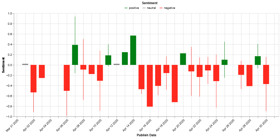
The application, despite its limitations, is primarily designed to enhance the visual analysis of brands. Therefore, I focused on presenting the search, sentiment, and topic analysis results in a clear and informative manner, utilizing both tables and plots. For instance, to allow users to access the original source material, I formatted the table displaying article headlines to include clickable URLs. For sentiment results, I used color-coded cells to provide an immediate visual understanding of the overall sentiment.

For plotting, I initially considered using matplotlib or seaborn. However, I quickly realized the importance of interactivity for data exploration. This led me to pivot towards Gradio Plots and finally Altair, which allowed me to create more engaging and interactive visualizations.

Deployment & UI

For the application’s user interface, I chose Gradio. Its simplicity in syntax for layout organization and its intuitive event handling with Blocks made development efficient. However, after extensive use, I encountered some limitations. Gradio’s native plotting options are relatively restricted, and the level of graph customization is limited. While embedding plots generated by other libraries is straightforward, these external plots don’t integrate as seamlessly as native Gradio components.

The entire application and its dependencies are containerized using Docker and deployed to Hugging Face Spaces. My experience with Docker for this project involved navigating some changes since my last container creation. Notably, I adopted uv as the Python package manager. Additionally, integrating libraries that require downloading data (such as nltk or Hugging Face models) presented initial challenges. While these issues ultimately proved solvable, they required persistent troubleshooting for a beginner like myself.

Final Thoughts

This project sparked several new ideas. One direction involves developing more nuanced methods for analyzing news bias, which could lead to deeper insight into media narratives. Another is expanding the scope of searches beyond specific brands to cover any topic of interest—an approach that holds great potential for OSINT analysts seeking broader situational awareness.

Smaller, specialized language models are very powerful when they’re used for tasks perfectly suited to their strengths. It became clear during the project that you don’t always need the largest, most complex models like GPT or Gemini. Sometimes, a smaller, focused model is more efficient, and there are even times when traditional NLP methods work best without any LLM at all.

A significant practical limitation was working within API usage quotas and limited hardware resources. Because the app depends on free API plans and CPU-only processing, there are strict caps on the number of requests and the volume of data it can handle. This naturally limits scalability.

🚀 Try the chatbot here!

The source code in the form of notebook and the data examples can be found here.