Distinguishing between real and imagined memories with Bayesian logistic regression

This brief research project was part of the course “Bayesian data analysis” in the Master in Methodology for behavioral sciences.

Description

In 2020, Sap et al. made an study in which they analyzed the content of real and imagined stories with Natural Language Processing techniques. The paper is quite interesting, but it is also possible to study the difference between the type of event (real/recalled or imagined) from a more conventional analytical approach. Here I propose to study the relationship between type of event and two of the variables collected, distraction during the writing of the story and the importance attributed to the event described.

A positive relationship is hypothesized between distraction and the probability that the narrated event will be remembered. In principle, creating a story should involve greater cognitive effort. Similarly, among those who write the event while being more distracted, it is expected that there will be a higher proportion of recalled events. On the other hand, the existence of a positive relationship between importance and the probability that the event is real is suggested. This hypothesis is based on the intuitive idea that it is more reasonable to attribute relevance to events or memories that are real, rather than simply imagined.

A convenient way to test our hypotheses is by fitting a logistic regression model. However, we are going to doing from a Bayesian perspective. Among other things that means we are going to consider the effects as random variables, not fixed constants. One benefit is that we can build probability (not confidence) intervals around the parameters. We will see later examples of this.

The complete model specification:

Each observation $i$ can correspond either to a a real event ($y_i=1$) or an imagined event ($y_i=0$) with probabilities $\pi_i$ and $1-\pi_i$ respectively. Note here that ${\bf y}$ and $\mathbf{\pi}$ are n-dimensional vectors because we have $n$ observations in the dataset. $$ y_i \sim Bernoulli(\pi_i) $$

Likelihood The probability of the type of event can be modeled by the logistic function. The predictors are ${\bf z}_1$ and ${\bf z}_2$, the standardized values of the attributes distraction and importance.

$$ \pi_i \sim Logistic(z_{1i},z_{2i};\beta_0,\beta_1,\beta_2) $$

Priors The specification of the prior beliefs about the parameters involved in regression is what makes the Bayesian approach different. Here I follow the recommendations of Gelman et al. (2008) to define weak informative prior distributions for the effect/slope of each variable and the intercept. It’s important to note that the scale parameter is a standard deviation, not a precision (the reciprocal).

$$ \beta_0 \sim Cauchy(0,10) $$

$$ \beta_1 \sim Cauchy(0,2.5) $$

$$ \beta_2 \sim Cauchy(0,2.5) $$

Parameter estimation (simplistic explanation)

In essence, Bayesian reasoning is about updating prior beliefs as more data is gathered. In our case, we want to update the different beliefs $p(\beta_j)$ to the posterior beliefs $p(\beta_j|data)$. One way to estimate this posterior distribution is by using Markov Chain Monte Carlo (MCMC) methods.They are approximate only

To see more about how MCMC was implemented you can check the report I made.

Summary of results

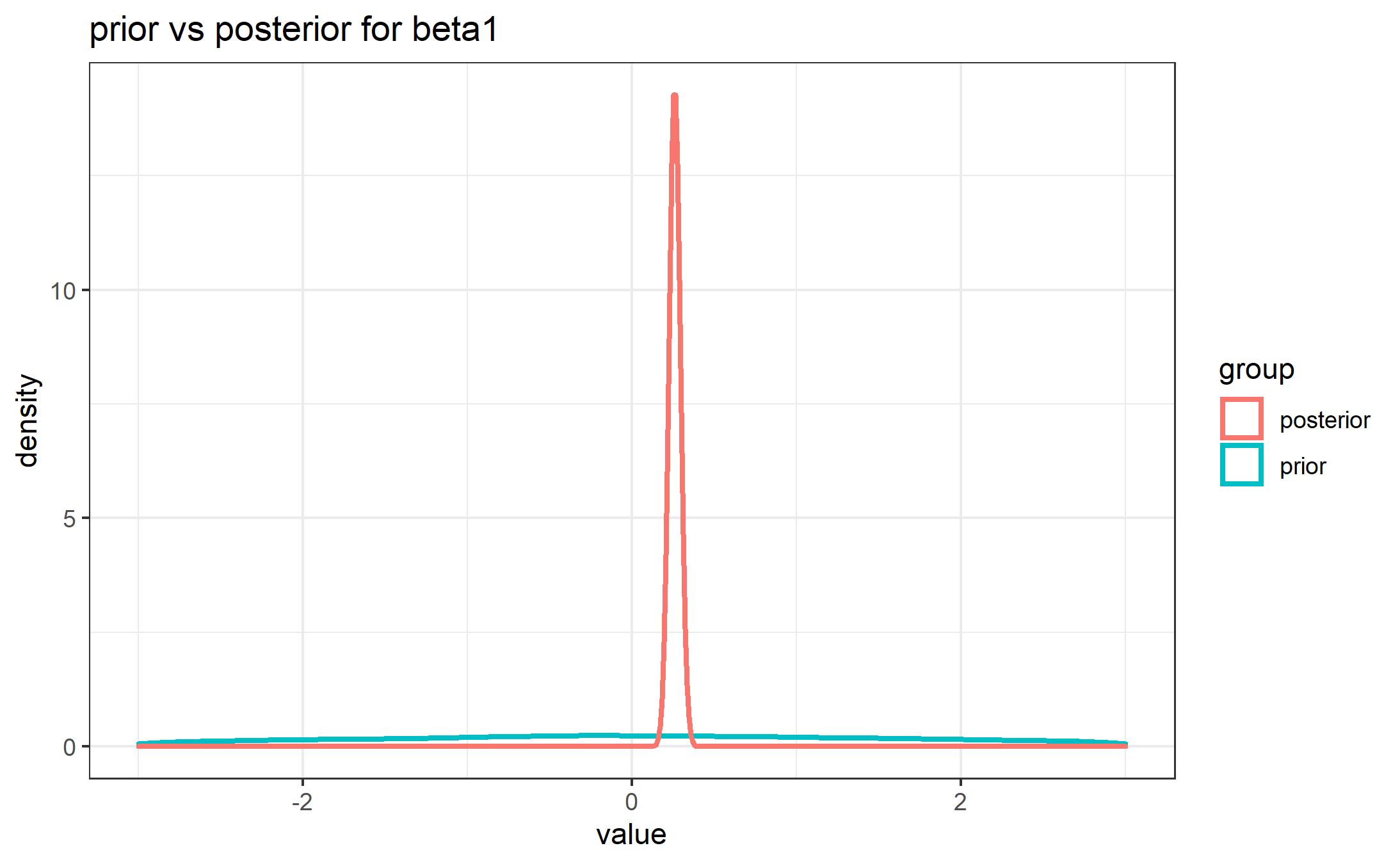
The result of the Bayesian inference can be easily visualized. In the next plot we see the case of the distraction effect. The blue curve represents prior “allocation of credibility across possibilities” (Kruschke, 2015). We chose a weakly informative prior, meaning that we didn’t assign much weight to any of the values possible for the effect of the distraction. However, after seeing the data, our belief about that variable changes. The red line represents the posterior density function, after the reallocation of credibility. Most probable values are around 0.2.

• In fact the 95% credible interval (see report) tells us that the effect of distraction lies, with a probability of 0.95, between 0.195 and 0.326, with mean 0.259. And what does mean? It indicates that the actual event odds increase 1.295 points for each extra z-score on the distraction variable, keeping the importance variable constant. For example, knowing that a subject scores very high on that trait (let us assume it is one standard deviation above the mean), we predict an average increase of 30% in the odds that the event described is real with respect to the “base” odds where we assume a mean value on distraction.

• With respect to $\beta_2$, it has a much larger average magnitude (1.382), with a 95% credible interval of (1.298, 1.469). Holding distraction constant, the odds of actual event increases by a factor of 3.982 for each standard deviation increase in the importance variable. Knowing that a subject considers the narrated story very important to him/her (scoring one standard deviation above the mean, for example), the probability goes from being approximately 0.5 (having assumed mean score in importance) to 0.79. All this considering the average value of $\beta_2$.

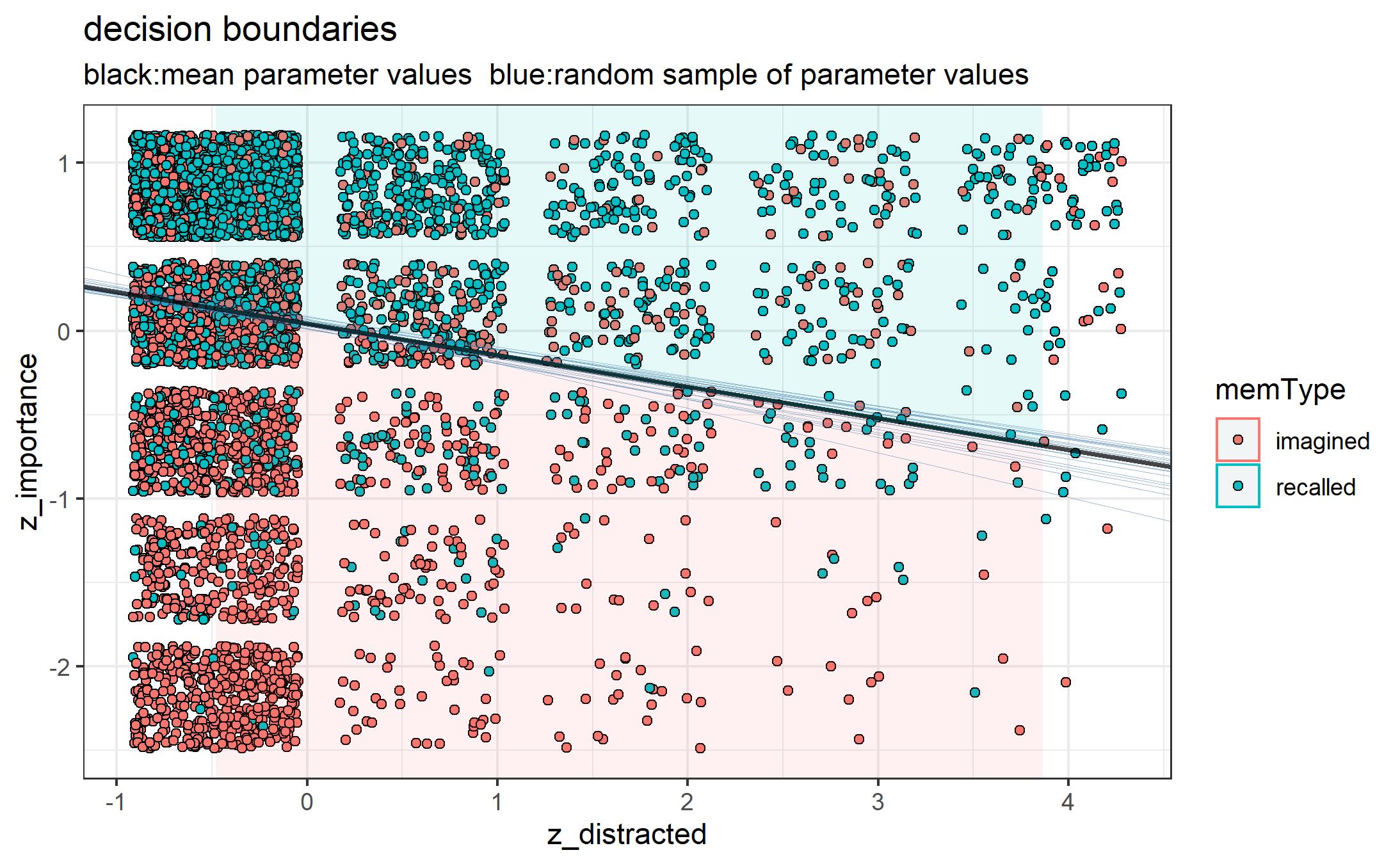
In terms of classification performance, the accuracy obtained was 0.73. But that value might not be reliable enough. It was computed using all the data available and taking the mean parameter values. The risk of overfitting is high. Assessing the performance of the model wasn’t the main goal though. In any case, this is the plot generated with some of the decision boundaries we would get with different values for the regression coefficients.

I know I’ve left out important information and results but you can check the complete report here. Also the appendix with the code and figures can be found here

References

Gelman, A., Jakulin, A., Pittau, M. G., & Su, Y. S. (2008). A weakly informative default prior distribution for logistic and other regression models. The annals of applied statistics, 2(4), 1360-1383.

Kruschke, J. (2015). Introduction: Credibility, Models,and Parameters. In J. Kruschke, Doing Bayesian data analysis: A tutorial with R, JAGS, and Stan (pp. 16-31). Elsevier.